基于MATLAB的数据处理与统计作图概要Word文件下载.docx

基于MATLAB的数据处理与统计作图概要Word文件下载.docx

《基于MATLAB的数据处理与统计作图概要Word文件下载.docx》由会员分享，可在线阅读，更多相关《基于MATLAB的数据处理与统计作图概要Word文件下载.docx（18页珍藏版）》请在冰豆网上搜索。

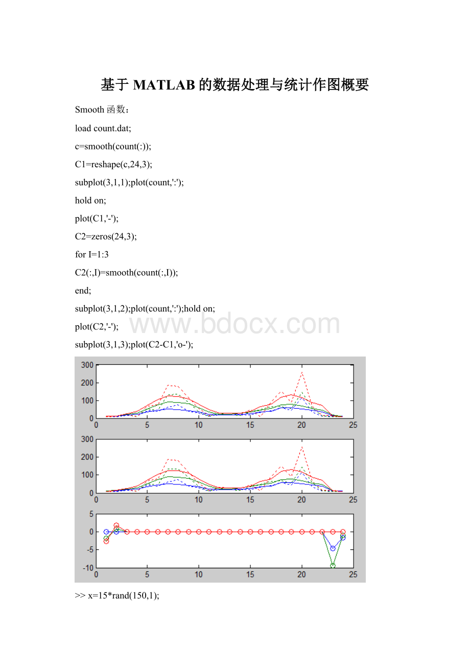
o-'

>

x=15*rand（150,1）;

y=sin（x）+0.5*（rand（size（x））-0.5）;

y（ceil（length（x）*rand（2,1）））=3;

noise=normrnd（0,15,150,1）;

y=y+noise;

yy1=smooth（x,y,0.1,'

loess'

yy2=smooth（x,y,0.1,'

rloess'

yy3=smooth（x,y,0.1,'

moving'

yy4=smooth（x,y,0.1,'

lowess'

yy5=smooth（x,y,0.1,'

sgolay'

yy6=smooth（x,y,0.1,'

rlowess'

[xx,ind]=sort（x）;

subplot（3,2,1）;

plot（xx,y（ind）,'

b-.'

xx,yy1（ind）,'

r-'

subplot（3,2,2）;

xx,yy2（ind）,'

subplot（3,2,3）;

xx,yy3（ind）,'

subplot（3,2,4）;

xx,yy4（ind）,'

subplot（3,2,5）;

xx,yy5（ind）,'

subplot（3,2,6）;

xx,yy6（ind）,'

Smoothts函数：

x=122+rand（500,4）;

p=x（:

4）'

;

out1=smoothts（p,'

b'

30）;

out2=smoothts（p,'

100）;

out3=smoothts（p,'

g'

out4=smoothts（p,'

100,100）;

out5=smoothts（p,'

e'

out6=smoothts（p,'

subplot（2,2,1）;

plot（p）;

subplot（2,2,2）;

plot（out1,'

k'

plot（out2,'

m.'

subplot（2,2,3）;

plot（out3,'

plot（out4,'

subplot（2,2,4）;

plot（out5,'

plot（out6,'

Medfilt1函数：

x=linspace（0,2*pi,250）'

y=sin（x）*150;

noise=normrnd（0,15,250,1）;

subplot（1,2,1）;

plot（x,y）;

yy=medfilt1（y,50）;

subplot（1,2,2）;

plot（x,y,'

r-.'

plot（x,yy,'

.'

直方图：

Hist函数：

x=randn（499,1）;

y=randn（499,3）;

hist（x）;

hist（x,100）;

hist（y,25）;

Histc函数：

x=-3.9:

0.1:

3.9;

y=randn（10000,1）;

hist（y,x）;

n=histc（y,x）;

c=cumsum（n）;

bar（x,c）;

Histfit函数：

r=normrnd（10,1,10,1）;

histfit（r）;

h=get（gca,'

Children'

盒子图：

N=1024;

x1=normrnd（5,1,N,1）;

x2=normrnd（6,1,N,1）;

x=[x1x2];

sym1='

*'

notch1=1;

boxplot（x,notch1,sym1）;

subplot（2,2,2）;

notch2=0;

boxplot（x,notch2）;

x=randn（100,25）;

subplot（2,1,1）;

boxplot（x）;

误差条图：

x=0:

pi/10:

pi;

y=sin（x）;

e=std（y）*ones（size（x））;

errorbar（x,y,e）

最小二乘法拟合直线：

x=1:

10;

y1=x+rand（1,10）;

scatter（x,y1,25,'

'

）

holdon;

y2=2*x+randn（1,10）;

plot（x,y2,'

mo'

y3=3*x+randn（1,10）;

plot（x,y3,'

rx:

y4=4*x+randn（1,10）;

plot（x,y4,'

g+--'

帕累托图：

codelines=[200120555608102410157687];

coders={'

Fred'

Ginger'

Norman'

Max'

Julia'

Wally'

Heidi'

Pat'

};

pareto（codelines,coders）

QQ图：

M=100;

N=1;

x=normrnd（0,1,M,N）;

y=rand（M,N）;

z=[x,y];

subplot（2,2,1）;

h1=qqplot（z）;

gridon;

x=normrnd（0,1,100,1）;

y=normrnd（0.5,2,50,1）;

h2=qqplot（x,y）;

x=normrnd（5,1,100,1）;

y=weibrnd（2,0.5,100,1）;

subplot（2,2,3）;

h3=qqplot（x,y）;

subplot（2,2,4）;

x=normrnd（10,1,100,1）;

qqplot（x）;

回归残差图：

X=[ones（10,1）（1:

10）'

];

y=X*[10;

1]+normrnd（0,0.1,10,1）;

[b,bint,r,rint]=regress（y,X,0.06）;

rcoplot（r,rint）;

多项式拟合曲线：

p=[1-2-10];

t=0:

3;

y=polyval（p,t）+0.5*randn（size（t））;

plot（t,y,'

ro'

h=refcurve（p）;

set（h,'

Color'

r'

q=polyfit（t,y,3）;

refcurve（q）;

参考线：

y=x+randn（1,10）;

scatter（x,y,25,'

lsline;

Noallowedlinetypesfound.Nothingdone.

mu=mean（y）;

hline=refline（[0mu]）;

set（hline,'

正态概率图：

h=normplot（z）;

点的标签：

loadcities;

education=ratings（:

6）;

arts=ratings（:

7）;

plot（education,arts,'

+'

gname（names）

工序能力指数：

data=normrnd（1,1,30,1）;

[p,cp,cpk]=capable（data,[-3,3]）

p=

0.0245

cp=

1.0284

cpk=

0.6562

规定区间的正态分布密度图：

p=normspec（[10Inf],11.5,1.25）;

标准差管理图：

loadparts;

schart（runout）;

均值管理图：

xbarplot（runout）;

gridon;