第二章 回归分析.docx

第二章 回归分析.docx

《第二章 回归分析.docx》由会员分享，可在线阅读，更多相关《第二章 回归分析.docx（35页珍藏版）》请在冰豆网上搜索。

第二章回归分析

第二节回归分析

2.1regress命令

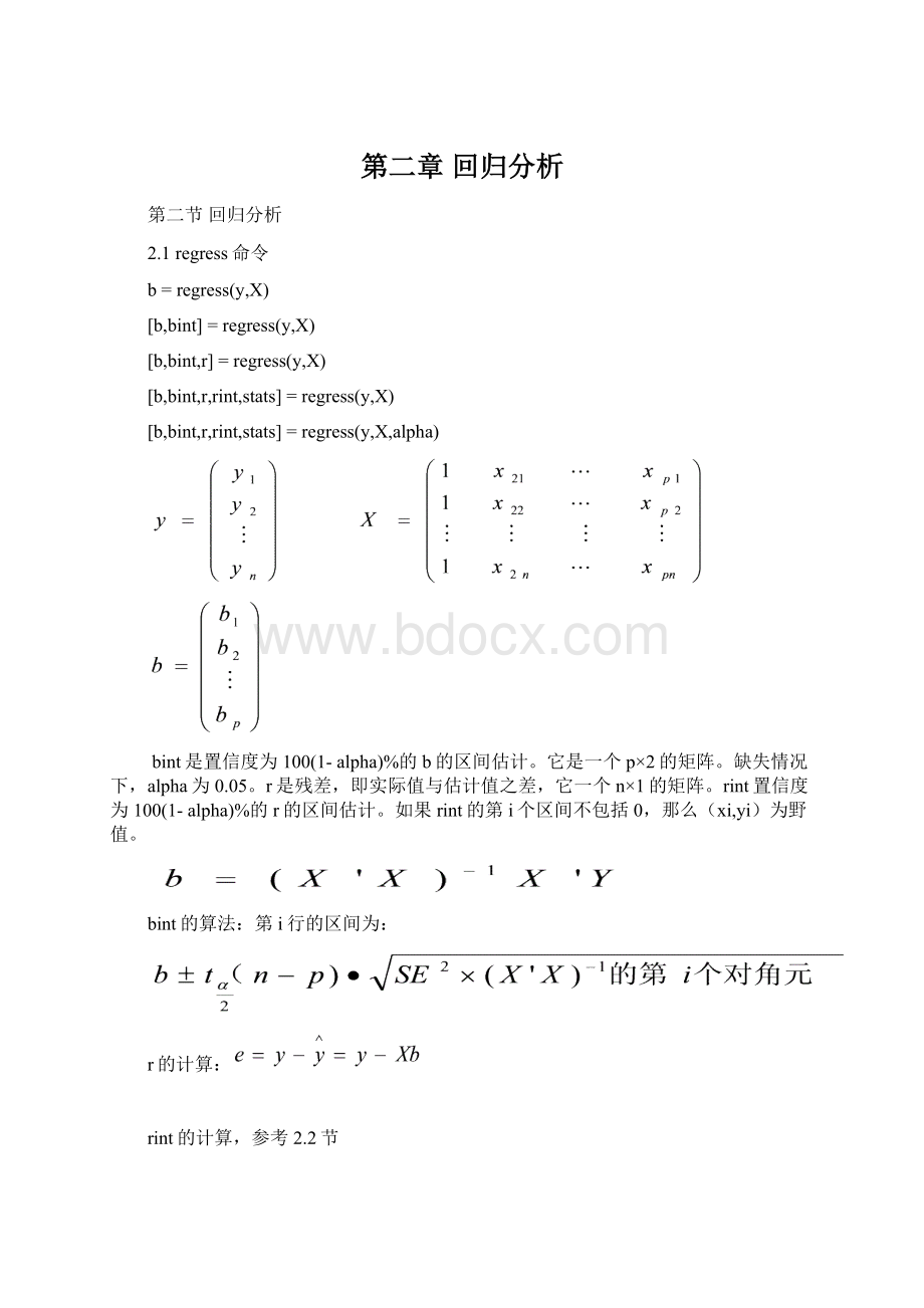
b=regress（y,X）

[b,bint]=regress（y,X）

[b,bint,r]=regress（y,X）

[b,bint,r,rint,stats]=regress（y,X）

[b,bint,r,rint,stats]=regress（y,X,alpha）

bint是置信度为100（1-alpha）%的b的区间估计。

它是一个p×2的矩阵。

缺失情况下，alpha为0.05。

r是残差，即实际值与估计值之差，它一个n×1的矩阵。

rint置信度为100（1-alpha）%的r的区间估计。

如果rint的第i个区间不包括0，那么（xi,yi）为野值。

bint的算法：

第i行的区间为：

r的计算：

rint的计算，参考2.2节

stats包括四项

1、可决系数

2、F值

3、F值对应的p值

注意这里是右侧检验的P值。

4、残差的方差

例子：

年次

1

2

3

4

5

6

7

8

9

10

销售量

Y

百件

10

10

15

13

14

20

18

24

19

23

居民人均收入

X2

百元

5

7

8

9

9

10

10

12

13

15

单价

X3

元

2

3

2

5

4

3

4

3

5

4

z=[10101513142018241923

578991010121315

2325434354];

z1=z';y=z1（:

1）;X=[ones（size（z,2）,1）z1（:

[2,3]）];

[b,bint,r,rint,stats]=regress（y,X,0.05）

b=

4.5875

1.8685

-1.7996

bint=

-1.371310.5463

1.23092.5060

-3.5327-0.0664

r=

-0.3307

-2.2681

-0.9361

0.5941

-0.2054

2.1265

1.9261

2.3896

-0.8797

-2.4162

rint=

-4.09963.4382

-6.18571.6495

-4.98283.1106

-2.93584.1241

-4.77874.3678

-2.05186.3048

-2.37556.2277

-1.16435.9434

-4.90303.1435

-5.12370.2912

stats=

0.879325.50370.00063.8685

下面讨论各值是怎么计算的：

b的计算：

b=inv（X'*X）*X'*y

b=

4.5875

1.8685

-1.7996

r的计算：

r=y-X*b

r=

-0.3307

-2.2681

-0.9361

0.5941

-0.2054

2.1265

1.9261

2.3896

-0.8797

-2.4162

rint的计算：

rint等于：

在本例中：

引用2.2节的studres

studres=

-0.2075

-1.3690

-0.5470

0.3980

-0.1062

1.2035

1.0588

1.5900

-0.5171

-2.1103

rint等于：

rint=[r-tinv（0.975,7）*r./studresr+tinv（0.975,7）*r./studres]

rint=

-4.09963.4382

-6.18571.6495

-4.98283.1106

-2.93584.1241

-4.77874.3678

-2.05186.3048

-2.37556.2277

-1.16435.9434

-4.90303.1435

-5.12370.2912

也可按此计算：

rint=[r-tinv（0.975,7）*sqrt（s2_i）.*sqrt（1-leverage）r+tinv（0.975,7）*sqrt（s2_i）.*sqrt（1-leverage）]

rint=

-4.09963.4382

-6.18571.6495

-4.98283.1106

-2.93584.1241

-4.77874.3678

-2.05186.3048

-2.37556.2277

-1.16435.9434

-4.90303.1435

-5.12370.2912

SE平方的计算：

sum（r.^2）/7

ans=

3.8685

bint的计算：

bint=[b+tinv（0.975,7）*sqrt（diag（3.8685*inv（X'*X）））b-tinv（0.975,7）*sqrt（diag（3.8685*inv（X'*X）））]

bint=

10.5463-1.3713

2.50601.2309

-0.0664-3.5327

R2的计算：

R2=1-sum（r.^2）/（var（y）*（length（y）-1））

R2=

0.8793

F值的计算：

F=（R2/2）/（（1-R2）/（10-3））

F=

25.5037

F值对应的P值

P=1-fcdf（25.5037,2,7）

P=

6.1045e-004

还可绘制残差图

rcoplot（r,rint）

每条线的上下两端对应于rint，中间的圆卷点对应于r。

如果某条线不通过中间的白线（即X轴），那么所对应的（xi,yi）为野值。

这个图中所有线条都通过X轴。

预测：

假设在未来五年，居民人均收入以4.5%的速度递增，而单价以1%的速度递减。

x1

（1）=15;

>>x2

（1）=4;

>>fori=1:

5

x1（i+1）=1.045*x1（i）;

x2（i+1）=0.99*x2（i）;

y（i+1）=4.5875+1.8685*x1（i+1）-1.7996*x2（i+1）;

end

yf=[x1;x2;y]

yf=

Columns1through4

15.000015.675016.380417.1175

4.00003.96003.92043.8812

026.749828.139129.5869

Columns5through6

17.887818.6927

3.84243.8040

31.096132.6693

最后一行为未来五年的预测值（0除外）。

2.2regstats线性回归诊断

2.2.1命令：

regstats（responses,data,model）

responses:

因变量，y它是n×1的列向量。

n为观察值个数。

data:

自变量，它是n×m的矩阵，m为自变量个数，注意它不包括全为1的列向量。

model:

modelcanbeoneofthefollowingstrings

'linear':

Includesconstantandlinearterms（default）.包括常数项和各变量。

'interaction':

Includesconstant,linear,andcrossproductterms.如自变量有两个时，X1，X2，则包括常数项、X1，X2，还有X1×X2。

'quadratic':

Includesinteractionsandsquaredterms.如自变量有两个时，X1，X2，则包括常数项、X1，X2，还有X1·X2、X12、X22。

'purequadratic':

Includesconstant,linear,andsquaredterms。

如自变量有两个时，X1，X2，则包括常数项、X1，X2，还有X12、X22。

regstats（responses,data,model）此命令将打开一个用户界面，包括以下20个统计量：

可参见《市场调查与分析》柯惠新丁立宏编著中国统计出版社2000.3第十二章

《统计手册》茆诗松主编科学出版社2003.1第十章

《统计建模与R软件》薛毅陈立萍清华大学出版社2007.4第六章

参考网站：

（1）QRDecomposition（Q）《矩阵论》程云鹏P206

X=Q×R，X包括全为1的列向量。

X为n×p的矩阵。

[Q,R]=qr（X,0）Q是n×p的矩阵，且满足Q'*Q=I

（2）QRDecomposition（R）

[Q,R]=qr（X,0）R是p×p的上三角形矩阵。

（3）RegressionCoefficients

beta=R\（Q'*y）即beta=inv（R）*（Q'*y）

把X=Q×R代入beta=inv（X'*X）*X'*y即得上式。

（4）FittedValuesoftheResponse

＝X*beta=X*inv（X'*X）*X'*y

（5）Residuals

（6）MeanSquaredError

（7）CovarianceMatrixofEstimatedCoefficients

（8）Hat（Projection）Matrix（帽子矩阵）

hatmat=Q*Q'yhat=hatmat*y

hatmat为n×n矩阵

将X=Q×R代入yhat=X*beta=X*inv（X'*X）*X'*y得：

yhat=Q*Q'*y

hatmat为投影矩阵。

（9）Leverage（中心化杠杆值）

leverage=diag（hatmat）=diag（Q*Q'）,它是n×1的列向量，n个值取值范围为[0，1]，第i值是度量第i的观察值在模型中的作用大小，如果第i个值越大，则在模型中的作用越大。

用leverage是寻找强影响点的一个办法。

所谓强影响点是指在模型中的作用特别大的点，就是说删除该点和不删除该点所得到的回归系数会有很差异的点。

理想的中心化杠杆值是每个杠杆值都具有相同的影响力，即所有的杠杆值都接近p/n，如果某个观测点的杠杆值大于等于2p/n，就认为它是一个强影响点。

（10）Delete-1Variance

它是除去第i个数据点后误差的方差的估计。

它是n×1的列向量。

s2_i=（（n-p）*mse-r.*r./（1-h））./（n-p-1）

1）nisthenumberofobservations.

2）pisthenumberofunknowncoefficients.

3）mseisthemeansquarederror.

4）risthevectorofresiduals.

5）histheleveragevector.

（11）Delete-1Coefficients

它是把第j个观察值删除后，所得回归系数矩阵。

它为p×n的矩阵，它的第j列对应的列向量是删除第i个观察值所得的回归系数。

b_i（:

j）=beta-Rinv*（Q（j,:

）.*r（j）./（1-h（j）））'

1）RinvistheinverseoftheRmatrix.

2）risthevectorofresiduals.

3）histheleveragevector.

（12）StandardizedResiduals

standres=r./sqrt（mse*（1-h））

1）risthevectorofresiduals.

2）mseisthemeansquarederror.

3）histheleveragevector.

Standres为n×1的列向量。

用它可以诊断异常点，异常点是指明显远离主体数据的观察点，表现为标准化残差（内学生化残差）过大的观测量，一般认为标准化残差绝对值大于2或3，则认为是异常点。

经典假设满足时，Standres（i）i=1、2、3…n，可近似看成独立同分布的，均服从标准正态分布

N（0，1）的随机变量。

如果大约有95%的点落在±2内，且没有任何明显的变化趋势，说明回归的基本假定满足，模型对于数据的拟合效果较好。

（13）StudentizedResiduals

studres=r./sqrt（s2_i*（1-h））

1）risthevectorofresiduals.

2）s2_iisthedelete-1variance.

3）histheleveragevector.

studres（i）i=1、2、3…n，经典假设满足时，服从自由度为n-p的t分布。

给定显著性水平

时，

则认为是异常点。

当n-p>30时，一般认为观察值所对应的学生化残差绝对值大于2或3，则认为是异常点。

（14）ScaledChangeinRegressionCoefficients

Thescaledchangeinregressioncoefficientsisap-by-nmatrix.Eachcolumncontainsthescaledchangeintheestimatedcoefficients,beta,causedbydeletingthecorrespondingobservation.

d=sqrt（diag（Rinv*Rinv'））;

dfbetas（:

j）=（beta-b_i（:

j））./（sqrt（s2_i（j）.*d（j））

1）RinvistheinverseoftheRmatrix.

2）b_iisthematrixofdelete-1coefficients.

3）s2_iisthevectorofdelete-1variances.

它是计算当某个观测点被排除后的回归系数的标准变化值，一般认为标准变化值大于

的点可能就是强影响点。

（15）ChangeinFittedValues

Thechangeinfittedvaluesisann-by-1vector.Eachelementcontainsthechangeinafittedvaluecausedbydeletingthecorrespondingobservation.

dffit=r.*（h./（1-h））

1）risthevectorofresiduals.

2）histheleveragevector.

表示删除某观察值后预测值的变化值。

（16）ScaledChangeinFittedValues

Thescaledchangeinfittedvaluesisann-by-1vector.Eachelementcontainsthechangeinafittedvaluecausedbydeletingthecorrespondingobservation,scaledbythestandarderror.

dffits=studres.*sqrt（h./（1-h））

1）studresisthevectorofstudentizedresiduals.

2）histheleveragevector.

它是计算当某个观察点被排除后的预测值的预测值的标准变化值，一般认为标准变化值的绝对值大于

的点可能就是强影响点。

（17）ChangeinCovariance

covr=1./（（（（n-p-1+studres.*studres）./（n-p））.^p）.*（1-h））

它是n×1的列向量。

1）nisthenumberofobservations.

2）pisthenumberofunknowncoefficients.

3）studresisthevectorofstudentizedresiduals.

4）histheleveragevector.

（18）Cook'sDistance

cookd=r.*r.*（h./（1-h）.^2）./（p*mse）risthevectorofresiduals.

1）histheleveragevector.

2）mseisthemeansquarederror.

3）pisthenumberofunknowncoefficients.

cookd是n×1的列向量，如果第i个值大于0.5，则第i个观察值可能为强影响点。

（19）Student'ststatistics

1）beta--Regressioncoefficientestimates

2）se--Standarderrorsfortheregressioncoefficientestimates

3）t--tstatisticsfortheregressioncoefficientestimates,eachoneforatestthatthecorrespondingcoefficientiszero

4）dfe--Degreesoffreedomforerror

5）pval--p-valuesforeachtstatistic,whichiscalculatedbythefollowingcode:

beta=R\（Q'*y）

se=sqrt（diag（covb））

t=beta./se

dfe=n-p

pval=2*（tcdf（-abs（t）,dfe））

（20）Fstatistic

1）sse--Errorsumofsquares

2）ssr--Regressionsumofsquares

3）dfe--Errordegreesoffreedom

4）dfr--Regressiondegreesoffreedom

5）f--Fstatisticvalue,foratestthatallregressioncoefficientsotherthantheconstanttermarezero

6）pval--p-valuefortheFstatistic,whichiscalculatedbythefollowingcode:

sse=norm（r）.^2

ssr=norm（yfit-mean（yfit））.^2

dfe=n-p

dfr=p-1

f=（ssr/dfr）/（sse/dfe）

pval=1-fcdf（f,dfr,dfe）

例子：

年次

1

2

3

4

5

6

7

8

9

10

销售量

Y

百件

10

10

15

13

14

20

18

24

19

23

居民人均收入

X2

百元

5

7

8

9

9

10

10

12

13

15

单价

X3

元

2

3

2

5

4

3

4

3

5

4

z=[10101513142018241923

578991010121315

2325434354];

z1=z';y=z1（:

1）;X=z1（:

[2,3]）;

regstats（y,X,'linear'）

在用户界面里全部选中得：

Q=

-0.3162-0.5449-0.1902

-0.3162-0.31790.0288

-0.3162-0.2043-0.4207

-0.3162-0.09080.6204

-0.3162-0.09080.2478

-0.31620.0227-0.2017

-0.31620.02270.1710

-0.31620.2497-0.3554

-0.31620.36330.3131

-0.31620.5903-0.2132

R=

-3.1623-30.9903-11.0680

08.80911.8163

002.6835

beta=

4.5875

1.8685

-1.7996

covb=

6.3503-0.3247-0.7947

-0.32470.0727-0.1108

-0.7947-0.11080.5372

yhat=

10.3307

12.2681

15.9361

12.4059

14.2054

17.8735

16.0739

21.6104

19.8797

25.4162

r=

-0.3307

-2.2681

-0.9361

0.5941

-0.2054

2.1265

1.9261

2.3896

-0.8797

-2.4162

mse=

3.8685

leverage=

0.4331

0.2019

0.3187

0.4932

0.1696

0.1412

0.1297

0.2887

0.3300

0.4939

sum（leverage）

ans=

3.0000

hatmat=

Columns1through8

0.43310.26770.29130.03150.10240.12600.05510.0315

0.26770.20190.15280.14670.13600.08700.09770.0104

0.29130.15280.3187-0.14240.01430.18020.02340.1985

0.03150.1467-0.14240.49320.2620-0.02720.2040-0.1