锁相环仿真基于MATLAB.docx
《锁相环仿真基于MATLAB.docx》由会员分享,可在线阅读,更多相关《锁相环仿真基于MATLAB.docx(15页珍藏版)》请在冰豆网上搜索。
锁相环仿真基于MATLAB
锁相环仿真
1.锁相环的理论分析
1.1锁相环的基本组成
锁相环路是一种反馈控制电路,简称锁相环(PLL,Phase-LockedLoop)。
锁相环的特点是:
利用外部输入的参考信号控制环路内部振荡信号的频率和相位。
因锁相环可以实现输出信号频率对输入信号频率的自动跟踪,所以锁相环通常用于闭环跟踪电路。
锁相环在工作的过程中,当输出信号的频率与输入信号的频率相等时,输出电压与输入电压保持固定的相位差值,即输出电压与输入电压的相位被锁住,这就是锁相环名称的由来。
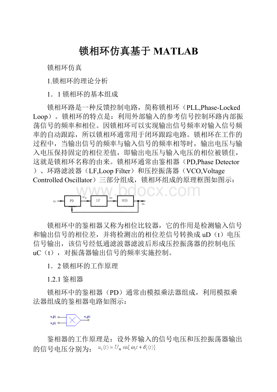
锁相环通常由鉴相器(PD,PhaseDetector)、环路滤波器(LF,LoopFilter)和压控振荡器(VCO,VoltageControlledOscillator)三部分组成,锁相环组成的原理框图如图示:
锁相环中的鉴相器又称为相位比较器,它的作用是检测输入信号和输出信号的相位差,并将检测出的相位差信号转换成uD(t)电压信号输出,该信号经低通滤波器滤波后形成压控振荡器的控制电压uC(t),对振荡器输出信号的频率实施控制。
1.2锁相环的工作原理
1.2.1鉴相器
锁相环中的鉴相器(PD)通常由模拟乘法器组成,利用模拟乘法器组成的鉴相器电路如图示:
鉴相器的工作原理是:
设外界输入的信号电压和压控振荡器输出的信号电压分别为:
式中的ω0为压控振荡器在输入控制电压为零或为直流电压时的振荡角频率,称为电路的固有振荡角频率。
则模拟乘法器的输出电压uD为:
1.2.2低通滤波器
低通滤波器(LF)的将上式中的和频分量滤掉,剩下的差频分量作为压控振荡器的输入控制电压uC(t)。
即uC(t)为:
式中的ωi为输入信号的瞬时振荡角频率,θi(t)和θO(t)分别为输入信号和输出信号的瞬时位相,根据相量的关系可得瞬时频率和瞬时位相的关系为:
即
则,瞬时相位差θd为
对两边求微分,可得频差的关系式为
上式等于零,说明锁相环进入相位锁定的状态,此时输出和输入信号的频率和相位保持恒定不变的状态,uc(t)为恒定值。
当上式不等于零时,说明锁相环的相位还未锁定,输入信号和输出信号的频率不等,uc(t)随时间而变。
1.2.3压控振荡器
压控振荡器(VCO)的压控特性如图示
该特性说明压控振荡器的振荡频率ωu以ω0为中心,随输入信号电压uc(t)线性地变化,变化的关系如下:
上式说明当uc(t)随时间而变时,压控振荡器(VCO)的振荡频率ωu也随时间而变,锁相环进入“频率牵引”,自动跟踪捕捉输入信号的频率,使锁相环进入锁定的状态,并保持ω0=ωi的状态不变。
2.信号流程图
锁相环的原理框图如下:
其工作过程如下:
(1)压控振荡器的输出Uo经过采集并分频;
(2)输出和基准信号同时输入鉴相器;
(3)鉴相器通过比较上述两个信号的频率差,然后输出一个直流脉冲电压Ud;
(4)Ud进入到滤波器里面,滤除高频成分后得到信息Ue;
(5)Ue进入到压控震荡器VCO里面,控制频率随输入电压线性地变化;
(6)这样经过一个很短的时间,VCO的输出就会稳定于某一期望值。
3.二阶环仿真源程序代码及仿真结果
3.1程序代码:
%File:
c6_nltvde.m
w2b=0;w2c=0;%initializeintegrators
yd=0;y=0;%initializedifferentialequation
tfinal=50;%simulationtime
fs=100;%samplingfrequency
delt=1/fs;%samplingperiod
npts=1+fs*tfinal;%numberofsamplessimulated
ydv=zeros(1,npts);%vectorofdy/dtsamples
yv=zeros(1,npts);%vectorofy(t)samples
%
%beginningofsimulationloop
fori=1:
npts
t=(i-1)*delt;%time
ift<20
ydd=4*exp(-t/2)-3*yd*abs(y)-9*y;%defort<20
else
ydd=4*exp(-t/2)-3*yd-9*y;%defort>=20
end
w1b=ydd+w2b;%firstintegrator-step1
w2b=ydd+w1b;%firstintegrator-step2
yd=w1b/(2*fs);%firstintegratoroutput
w1c=yd+w2c;%secondintegrator-step1
w2c=yd+w1c;%secondintegrator-step2
y=w1c/(2*fs);%secondintegratoroutput
ydv(1,i)=yd;%builddy/dtvector
yv(1,i)=y;%buildy(t)vector
end%endofsimulationloop
plot(yv,ydv)%plotphaseplane
xlabel('y(t)')%labelxaxis
ylabel('dy/dt')%labelyzxis
%Endofscriptfile.
%File:
pllpost.m
%
kk=0;
whilekk==0
k=menu('PhaseLockLoopPostprocessor',...
'InputFrequencyandVCOFrequency',...
'InputPhaseandVCOPhase',...
'FrequencyError','PhaseError','PhasePlanePlot',...
'PhasePlaneandTimeDomainPlots','ExitProgram');
ifk==1
plot(t,fin,'k',t,fvco,'k')
title('InputFrequencyandVCOFreqeuncy')
xlabel('Time-Seconds');ylabel('Frequency-Hertz');pause
elseifk==2
pvco=phin-phierror;plot(t,phin,t,pvco)
title('InputPhaseandVCOPhase')
xlabel('Time-Seconds');ylabel('Phase-Radians');pause
elseifk==3
plot(t,freqerror);title('FrequencyError')
xlabel('Time-Seconds');ylabel('FrequencyError-Hertz');pause
elseifk==4
plot(t,phierror);title('PhaseError')
xlabel('Time-Seconds');ylabel('PhaseError-Radians');pause
elseifk==5
ppplot
elseifk==6
subplot(211);phierrn=phierror/pi;
plot(phierrn,freqerror,'k');grid;
title('PhasePlanePlot');xlabel('PhaseError/Pi');
ylabel('FrequencyError-Hertz');subplot(212)
plot(t,fin,'k',t,fvco,'k');grid
title('InputFrequencyandVCOFreqeuncy')
xlabel('Time-Seconds');ylabel('Frequency-Hertz');subplot(111)
elseifk==7
kk=1;
endend%Endofscriptfile.
%File:
pllpre.m
%
clearall%besafe
disp('')%insertblankline
fdel=input('EnterthesizeofthefrequencystepinHertz>');
fn=input('EntertheloopnaturalfrequencyinHertz>');
lambda=input('Enterlambda,therelativepoleoffset>');
disp('')
disp('Acceptdefaultvalues:
')
disp('zeta=1/sqrt
(2)=0.707,')
disp('fs=200*fn,and')
disp('tstop=1')
dtype=input('Enteryforyesornforno>','s');
ifdtype=='y'
zeta=1/sqrt
(2);
fs=200*fn;
tstop=1;
else
zeta=input('Enterzeta,theloopdampingfactor>');
fs=input('EnterthesamplingfrequencyinHertz>');
tstop=input('Entertstop,thesimulationruntime>');
end%
npts=fs*tstop+1;%numberofsimulationpoints
t=(0:
(npts-1))/fs;%defaulttimevector
nsettle=fix(npts/10);%setnsettletimeas0.1*npts
tsettle=nsettle/fs;%settsettle
%Thenexttwolinesestablishtheloopinputfrequencyandphase
%deviations.
fin=[zeros(1,nsettle),fdel*ones(1,npts-nsettle)];
phin=[zeros(1,nsettle),2*pi*fdel*t(1:
(npts-nsettle))];
disp('')%insertblankline
%endofscriptfilepllpre.m
%File:
pll2sin.m
w2b=0;w2c=0;s5=0;phivco=0;%initialize
twopi=2*pi;%define2*pi
twofs=2*fs;%define2*fs
G=2*pi*fn*(zeta+sqrt(zeta*zeta-lambda));%setloopgain
a=2*pi*fn/(zeta+sqrt(zeta*zeta-lambda));%setfilterparameter
a1=a*(1-lambda);a2=a*lambda;%defineconstants
phierror=zeros(1,npts);%initializevector
fvco=zeros(1,npts);%initializevector
%beginningofsimulationloop
fori=1:
npts
s1=phin(i)-phivco;%phaseerror
s2=sin(s1);%sinusoidalphasedetector
s3=G*s2;
s4=a1*s3;
s4a=s4-a2*s5;%loopfilterintegratorinput
w1b=s4a+w2b;%filterintegrator(step1)
w2b=s4a+w1b;%filterintegrator(step2)
s5=w1b/twofs;%generatefiteroutput
s6=s3+s5;%VCOintegratorinput
w1c=s6+w2c;%VCOintegrator(step1)
w2c=s6+w1c;%VCOintegrator(step2)
phivco=w1c/twofs;%generateVCOoutput
phierror(i)=s1;%buildphaseerrorvector
fvco(i)=s6/twopi;%buildVCOinputvector
end
%endofsimulationloop
freqerror=fin-fvco;%buildfrequencyerrorvector
%Endofscriptfile.
function[]=pplane(x,y,nsettle)
%Plotsthephaseplanewithphaseintherange(-pi,pi)
ln=length(x);
maxfreq=max(y);
minfreq=min(y);
close%Oldfigurediscarded
axis([-111.1*minfreq1.1*maxfreq]);%Establishscale
holdon%Collectinfofornewfig
j=nsettle;
whileji=1;
whilex(j)a(i)=x(j)/pi;
b(i)=y(j);
j=j+1;
i=i+1;
end
plot(a,b,'k')
a=[];
b=[];
x=x-2*pi;
end
holdoff
title('Phase-PlanePlot')
xlabel('PhaseError/Pi')
ylabel('FrequencyErrorinHertz')
grid%Endofscriptfile.
%File:
ppplot.m
%ppplot.misthescriptfileforplottingphaseplaneplots.Ifthe
%phaseplaneisconstrainedto(-pi,pi)ppplot.mcallspplane.m.
kz=0;
whilekz==0
k=menu('PhasePlaneOptions',...
'ExtendedPhasePlane',...
'PhasePlanemod(2pi)',...
'ExitPhasePlaneMenu');
ifk==1
phierrn=phierrn/pi;
plot(phierrn,freqerror,'k')
title('PhasePlanePlot')
xlabel('PhaseError/Pi')
ylabel('FrequencyError-Hertz')
grid
pause
elseifk==2
pplane(phierrn,freqerror,nsettle+1)
pause
elseifk==3
kz=1;
end
end%Endofscriptfile.
3.2仿真结果:
G=30时的仿真图形:
Acceptthetentativevalues:
thefirstloopfrequencyis5
Enteryforyesornforno>y
Entertheloopgain>30输入环路增益为30
EnterthesamplingfrequencyinHertz>1200
Entertstop,thesimulationruntime>5仿真时间为5秒
相平面图输入频率和VCO频率图
输入相位和VCO相位图频率差图
相位差图
G=40时的仿真图形:
Acceptthetentativevalues:
thefirstloopfrequencyis5
Enteryforyesornforno>y
Entertheloopgain>40输入环路增益为40
EnterthesamplingfrequencyinHertz>1200
Entertstop,thesimulationruntime>5仿真时间为5秒
相平面图输入频率和VCO频率图
相位差图频率差图
输入频率和VCO频率图输入相位和VCO相位图
 升级会员
升级会员 