中级计量经济学第四章习题以及解答思路EViews.docx
《中级计量经济学第四章习题以及解答思路EViews.docx》由会员分享,可在线阅读,更多相关《中级计量经济学第四章习题以及解答思路EViews.docx(20页珍藏版)》请在冰豆网上搜索。
中级计量经济学第四章习题以及解答思路EViews
第4章
习题一
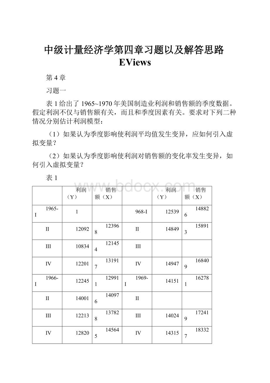
表1给出了1965~1970年美国制造业利润和销售额的季度数据。
假定利润不仅与销售额有关,而且和季度因素有关。
要求对下列二种情况分别估计利润模型:
(1)如果认为季度影响使利润平均值发生变异,应如何引入虚拟变量?
(2)如果认为季度影响使利润对销售额的变化率发生变异,如何引入虚拟变量?
表1
利润(Y)
销售额(X)
利润(Y)
销售额(X)
1965-I
1
968-I
12539
148826
II
12092
123968
II
14849
158913
III
10834
121454
III
IV
12201
131917
IV
14947
168409
1966-I
12245
129911
1969-I
14151
162781
II
14001
140976
II
III
12213
137828
III
14024
172419
IV
12820
145645
IV
14315
183327
1967-I
1
970-I
12381
170415
II
12615
145126
II
III
11014
141536
III
12174
176712
IV
12730
151776
IV
10985
180370
Quarterly65-70
Quick-EquationEstimation
Ycx@seas
(1)@seas
(2)@seas(3)
DependentVariable:
Y
Method:
LeastSquares
Date:
11/26/14Time:
18:
38
Sample:
1965Q11970Q4
Includedobservations:
24
Variable
Coefficient
Std.Error
t-Statistic
Prob.
C
6868.015
1892.766
3.628559
0.0018
X
0.038265
0.011483
3.332252
0.0035
@SEAS
(1)
-182.1690
654.3568
-0.278394
0.7837
@SEAS
(2)
1140.294
630.6806
1.808038
0.0865
@SEAS(3)
-400.3371
636.1128
-0.629349
0.5366
R-squared
0.525596
Meandependentvar
12838.54
AdjustedR-squared
0.425721
S.D.dependentvar
1433.284
S.E.ofregression
1086.160
Akaikeinfocriterion
17.00174
Sumsquaredresid
Schwarzcriterion
17.24716
Loglikelihood
-199.0208
F-statistic
5.262563
Durbin-Watsonstat
0.388380
Prob(F-statistic)
0.005024
T和P在5%情况下都不通过,第二季度相对还好一点
假设第二季度显著,结果的经济含义是什么?
Ycx@seas
(2)@seas(3)@seas(4)
DependentVariable:
Y
Method:
LeastSquares
Date:
11/26/14Time:
18:
47
Sample:
1965Q11970Q4
Includedobservations:
24
Variable
Coefficient
Std.Error
t-Statistic
Prob.
C
6685.846
1711.618
3.906155
0.0009
X
0.038265
0.011483
3.332252
0.0035
@SEAS
(2)
1322.463
638.4258
2.071444
0.0522
@SEAS(3)
-218.1681
632.1991
-0.345094
0.7338
@SEAS(4)
182.1690
654.3568
0.278394
0.7837
R-squared
0.525596
Meandependentvar
12838.54
AdjustedR-squared
0.425721
S.D.dependentvar
1433.284
S.E.ofregression
1086.160
Akaikeinfocriterion
17.00174
Sumsquaredresid
Schwarzcriterion
17.24716
Loglikelihood
-199.0208
F-statistic
5.262563
Durbin-Watsonstat
0.388380
Prob(F-statistic)
0.005024
第二季度依旧显著影响
四种都试一下(去掉一个季节),选一个最显著的
124
DependentVariable:
Y
Method:
LeastSquares
Date:
11/26/14Time:
18:
51
Sample:
1965Q11970Q4
Includedobservations:
24
Variable
Coefficient
Std.Error
t-Statistic
Prob.
C
6467.678
1789.178
3.614888
0.0018
X
0.038265
0.011483
3.332252
0.0035
@SEAS
(1)
218.1681
632.1991
0.345094
0.7338
@SEAS
(2)
1540.632
628.3419
2.451900
0.0241
@SEAS(4)
400.3371
636.1128
0.629349
0.5366
R-squared
0.525596
Meandependentvar
12838.54
AdjustedR-squared
0.425721
S.D.dependentvar
1433.284
S.E.ofregression
1086.160
Akaikeinfocriterion
17.00174
Sumsquaredresid
Schwarzcriterion
17.24716
Loglikelihood
-199.0208
F-statistic
5.262563
Durbin-Watsonstat
0.388380
Prob(F-statistic)
0.005024
134
DependentVariable:
Y
Method:
LeastSquares
Date:
11/26/14Time:
18:
52
Sample:
1965Q11970Q4
Includedobservations:
24
Variable
Coefficient
Std.Error
t-Statistic
Prob.
C
8008.309
1827.543
4.382009
0.0003
X
0.038265
0.011483
3.332252
0.0035
@SEAS
(1)
-1322.463
638.4258
-2.071444
0.0522
@SEAS(3)
-1540.632
628.3419
-2.451900
0.0241
@SEAS(4)
-1140.294
630.6806
-1.808038
0.0865
R-squared
0.525596
Meandependentvar
12838.54
AdjustedR-squared
0.425721
S.D.dependentvar
1433.284
S.E.ofregression
1086.160
Akaikeinfocriterion
17.00174
Sumsquaredresid
Schwarzcriterion
17.24716
Loglikelihood
-199.0208
F-statistic
5.262563
Durbin-Watsonstat
0.388380
Prob(F-statistic)
0.005024
(2)
Y=c+βx+α1D1X+α2D2X+α3D3X
D1=1(第一季度)0(其他)
Ycx@seas
(1)*x@seas
(2)*x@seas(3)*x
DependentVariable:
Y
Method:
LeastSquares
Date:
11/26/14Time:
19:
00
Sample:
1965Q11970Q4
Includedobservations:
24
Variable
Coefficient
Std.Error
t-Statistic
Prob.
C
6965.852
1753.642
3.972220
0.0008
X
0.037363
0.011139
3.354215
0.0033
@SEAS
(1)*X
-0.000893
0.004259
-0.209588
0.8362
@SEAS
(2)*X
0.007712
0.003962
1.946502
0.0665
@SEAS(3)*X
-0.002291
0.004041
-0.566985
0.5774
R-squared
0.528942
Meandependentvar
12838.54
AdjustedR-squared
0.429771
S.D.dependentvar
1433.284
S.E.ofregression
1082.323
Akaikeinfocriterion
16.99466
Sumsquaredresid
Schwarzcriterion
17.24009
Loglikelihood
-198.9359
F-statistic
5.333675
Durbin-Watsonstat
0.418713
Prob(F-statistic)
0.004722
DependentVariable:
Y
Method:
LeastSquares
Date:
11/26/14Time:
19:
10
Sample:
1965Q11970Q4
Includedobservations:
24
Variable
Coefficient
Std.Error
t-Statistic
Prob.
C
8008.309
1827.543
4.382009
0.0003
X
0.038265
0.011483
3.332252
0.0035
@SEAS
(1)
-1322.463
638.4258
-2.071444
0.0522
@SEAS(3)
-1540.632
628.3419
-2.451900
0.0241
@SEAS(4)
-1140.294
630.6806
-1.808038
0.0865
R-squared
0.525596
Meandependentvar
12838.54
AdjustedR-squared
0.425721
S.D.dependentvar
1433.284
S.E.ofregression
1086.160
Akaikeinfocriterion
17.00174
Sumsquaredresid
Schwarzcriterion
17.24716
Loglikelihood
-199.0208
F-statistic
5.262563
Durbin-Watsonstat
0.388380
Prob(F-statistic)
0.005024
DependentVariable:
Y
Method:
LeastSquares
Date:
11/26/14Time:
19:
11
Sample:
1965Q11970Q4
Includedobservations:
24
Variable
Coefficient
Std.Error
t-Statistic
Prob.
C
6965.852
1753.642
3.972220
0.0008
X
0.035072
0.011790
2.974675
0.0078
@SEAS
(1)*X
0.001398
0.004241
0.329736
0.7452
@SEAS
(2)*X
0.010003
0.004068
2.458823
0.0237
@SEAS(4)*X
0.002291
0.004041
0.566985
0.5774
R-squared
0.528942
Meandependentvar
12838.54
AdjustedR-squared
0.429771
S.D.dependentvar
1433.284
S.E.ofregression
1082.323
Akaikeinfocriterion
16.99466
Sumsquaredresid
Schwarzcriterion
17.24009
Loglikelihood
-198.9359
F-statistic
5.333675
Durbin-Watsonstat
0.418713
Prob(F-statistic)
0.004722
DependentVariable:
Y
Method:
LeastSquares
Date:
11/26/14Time:
19:
11
Sample:
1965Q11970Q4
Includedobservations:
24
Variable
Coefficient
Std.Error
t-Statistic
Prob.
C
6965.852
1753.642
3.972220
0.0008
X
0.036471
0.012353
2.952415
0.0082
@SEAS
(2)*X
0.008604
0.004237
2.030539
0.0565
@SEAS(3)*X
-0.001398
0.004241
-0.329736
0.7452
@SEAS(4)*X
0.000893
0.004259
0.209588
0.8362
R-squared
0.528942
Meandependentvar
12838.54
AdjustedR-squared
0.429771
S.D.dependentvar
1433.284
S.E.ofregression
1082.323
Akaikeinfocriterion
16.99466
Sumsquaredresid
Schwarzcriterion
17.24009
Loglikelihood
-198.9359
F-statistic
5.333675
Durbin-Watsonstat
0.418713
Prob(F-statistic)
0.004722
习题二
表2给出了某地区某行业的库存
和销售
的统计资料。
假设库存额依赖于本年销售额与前三年的销售额,试用Almon变换估计以下有限分布滞后模型:
表2
库存Y
(万元)
销售额X
(万元)
库存Y
(万元)
销售额X
(万元)
1980
11267
8827
1990
17053
13668
1981
12661
9247
1991
19491
14956
1982
12968
9579
1992
21164
15483
1983
12518
9
9
16761
1984
13177
10
9
17852
1985
13454
10265
1995
25411
17620
1986
13735
10299
1996
25611
18639
1987
14553
11
0
20672
1988
15011
11677
1998
30218
23799
1989
15846
12445
1999
36784
27359
Y=α+α0ΣXt-i+α1ΣXt-i+α2ΣXt-i+μt
↑3,i=0笔记11,26)
在最上面输入
genrz0=x+x(-1)+x(-1)+x(-3)
genrz1=x(-1)+2*x(-2)+3*x(-3)
genrz2=x(-1)+4*x(-2)+9*x(-3)
ycz0z1z2
DependentVariable:
Y
Method:
LeastSquares
Date:
11/26/14Time:
19:
38
Sample(adjusted):
19831999
Includedobservations:
17afteradjustments
Variable
Coefficient
Std.Error
t-Statistic
Prob.
C
-1928.495
503.5272
-3.829972
0.0021
Z0
0.344027
0.091848
3.745615
0.0024
Z1
0.815758
0.351519
2.320667
0.0372
Z2
-0.339041
0.128632
-2.635739
0.0206
R-squared
0.996564
Meandependentvar
20467.29
AdjustedR-squared
0.995771
S.D.dependentvar
6997.995
S.E.ofregression
455.0907
Akaikeinfocriterion
15.28119
Sumsquaredresid
2692398.
Schwarzcriterion
15.47724
Loglikelihood
-125.8902
F-statistic
1256.768
Durbin-Watsonstat
1.985515
Prob(F-statistic)
0.000000
YcPDL(x,3,2)
重新回归
DependentVariable:
Y
Method:
LeastSquares
Date:
11/26/14Time:
19:
46
Sample(adjusted):
19831999
Includedobservations:
17afteradjustments
Variable
Coefficient
Std.Error
t-Statistic
Prob.
C
-1784.821
498.4654
-3.5806
 升级会员
升级会员 