计量经济学国债发行额数学模型.docx
《计量经济学国债发行额数学模型.docx》由会员分享,可在线阅读,更多相关《计量经济学国债发行额数学模型.docx(14页珍藏版)》请在冰豆网上搜索。
计量经济学国债发行额数学模型
国债,又称国家公债,是国家以其信用为基础,按照债的一般原则,通过向社会筹集资金所形成的债权债务关系。
国债是由国家发行的债券,是中央政府为筹集财政资金而发行的一种政府债券,是中央政府向投资者出具的、承诺在一定时期支付利息和到期偿还本金的债权债务凭证,由于国债的发行主体是国家,所以它具有最高的信用度,被公认为是最安全的投资工具。
国债售出或被个人和企业认购的过程,它是国债运行的起点和基础环节,核心是确定国债售出的方式即国债发行方式。
一般而言,国债发行主要有四种方式:
1.固定收益出售法;
2.公募拍卖方式。
3.连续经销方式
4.承受发行法
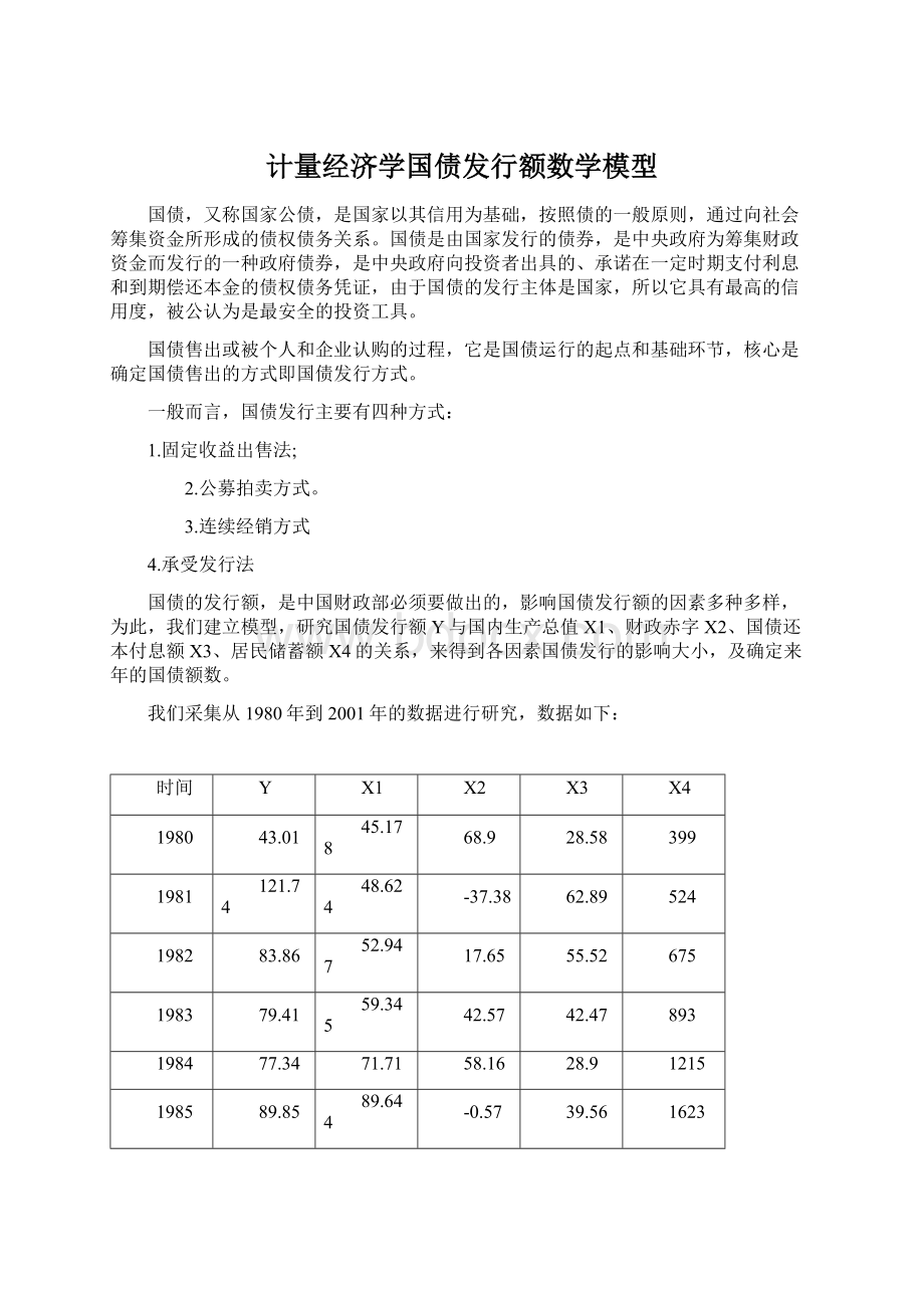
国债的发行额,是中国财政部必须要做出的,影响国债发行额的因素多种多样,为此,我们建立模型,研究国债发行额Y与国内生产总值X1、财政赤字X2、国债还本付息额X3、居民储蓄额X4的关系,来得到各因素国债发行的影响大小,及确定来年的国债额数。
我们采集从1980年到2001年的数据进行研究,数据如下:
时间
Y
X1
X2
X3
X4
1980
43.01
45.178
68.9
28.58
399
1981
121.74
48.624
-37.38
62.89
524
1982
83.86
52.947
17.65
55.52
675
1983
79.41
59.345
42.57
42.47
893
1984
77.34
71.71
58.16
28.9
1215
1985
89.85
89.644
-0.57
39.56
1623
1986
138.25
102.022
82.9
50.17
2237
1987
223.55
119.625
62.83
79.83
3081
1988
270.78
149.283
133.97
76.76
3822
1989
407.97
169.092
158.88
72.37
5196
1990
375.45
185.479
146.49
190.07
7120
1991
461.4
216.178
237.14
246.8
9242
1992
669.68
266.381
258.83
438.57
11759
1993
739.22
346.344
293.35
336.22
15204
1994
1175.25
467.594
574.52
499.36
21519
1995
1549.76
584.781
581.52
882.96
29662
1996
1967.28
678.846
529.56
1355.03
38521
1997
2476.82
744.626
582.42
1918.37
46280
1998
3310.93
783.452
922.23
2352.92
53408
1999
3715.03
820.6746
1743.59
1910.53
59622
2000
4180.1
894.422
2491.27
1579.82
64332
2001
4604
959.333
2516.54
2007.73
73762
由数据,我们进行第一次拟合:
DependentVariable:
Y
Method:
LeastSquares
Date:
10/25/11Time:
16:
54
Sample:
19802001
Includedobservations:
22
Variable
Coefficient
Std.Error
t-Statistic
Prob.
C
14.43481
35.40908
0.407658
0.6886
X1
0.190236
0.450990
0.421818
0.6784
X2
0.940201
0.153877
6.110072
0.0000
X3
0.820870
0.168306
4.877234
0.0001
X4
0.005481
0.014937
0.366969
0.7182
R-squared
0.998963
Meandependentvar
1216.395
AdjustedR-squared
0.998719
S.D.dependentvar
1485.993
S.E.ofregression
53.18111
Akaikeinfocriterion
10.98200
Sumsquaredresid
48079.92
Schwarzcriterion
11.22996
Loglikelihood
-115.8020
F-statistic
4094.752
Durbin-Watsonstat
2.072804
Prob(F-statistic)
0.000000
得到线性拟合方程为:
Y=14.43481+0.190236X1+0.940201X2+0.820870X3+0.005481X4
O.4076580.4218186.1100724.8772340.366969
=O.9989630.998719F=4094.752
从总体上看,模型中国债发行额与各解释变量线性关系显著。
检验:
计算解释变量之间的简单相关系数
X1
X2
X3
X4
X1
1.000000
0.869643
0.954508
0.986413
X2
0.869643
1.000000
0.787957
0.919614
X3
0.954508
0.787957
1.000000
0.959852
X4
0.986413
0.919614
0.959852
1.000000
从表中,可以发现,解释变量存在着高度线性相关,虽然在整体上线性回归拟合较好,但X1,X4的参数t值并不显著,表明模型中解释变量存在严重多重线性共线性。
修正:
1、Y与X1线性回归:
DependentVariable:
Y
Method:
LeastSquares
Date:
10/25/11Time:
17:
16
Sample:
19802001
Includedobservations:
22
Variable
Coefficient
Std.Error
t-Statistic
Prob.
C
-388.3980
124.1492
-3.128479
0.0053
X1
4.494313
0.261595
17.18041
0.0000
R-squared
0.936541
Meandependentvar
1216.395
AdjustedR-squared
0.933369
S.D.dependentvar
1485.993
S.E.ofregression
383.5804
Akaikeinfocriterion
14.82348
Sumsquaredresid
2942679.
Schwarzcriterion
14.92267
Loglikelihood
-161.0583
F-statistic
295.1665
Durbin-Watsonstat
0.248664
Prob(F-statistic)
0.000000
Y=-388.3980+4.494313X1
-3.12847917.18041
=0.9365410.933369F=295.1665
2、Y与X2拟合:
DependentVariable:
Y
Method:
LeastSquares
Date:
10/25/11Time:
17:
21
Sample:
19802001
Includedobservations:
22
Variable
Coefficient
Std.Error
t-Statistic
Prob.
C
249.5863
129.5995
1.925827
0.0685
X2
1.855133
0.143221
12.95296
0.0000
R-squared
0.893492
Meandependentvar
1216.395
AdjustedR-squared
0.888166
S.D.dependentvar
1485.993
S.E.ofregression
496.9387
Akaikeinfocriterion
15.34132
Sumsquaredresid
4938962.
Schwarzcriterion
15.44050
Loglikelihood
-166.7545
F-statistic
167.7791
Durbin-Watsonstat
0.617461
Prob(F-statistic)
0.000000
Y=249.5863+1.855133X2
1.92582712.95296
=0.8934920.888166F=167.7791
3、Y与X3拟合:
DependentVariable:
Y
Method:
LeastSquares
Date:
10/25/11Time:
17:
27
Sample:
19802001
Includedobservations:
22
Variable
Coefficient
Std.Error
t-Statistic
Prob.
C
80.25663
138.5002
0.579469
0.5687
X3
1.753369
0.136369
12.85750
0.0000
R-squared
0.892076
Meandependentvar
1216.395
AdjustedR-squared
0.886680
S.D.dependentvar
1485.993
S.E.ofregression
500.2312
Akaikeinfocriterion
15.35453
Sumsquaredresid
5004625.
Schwarzcriterion
15.45371
Loglikelihood
-166.8998
F-statistic
165.3154
Durbin-Watsonstat
0.652788
Prob(F-statistic)
0.000000
Y=80.25663+1753369X3
0.57946912.85750
=0.8920760.886680F=165.3154
因常数项t=0.579469<2.306则省略常数项,得到拟合方程为:
Y=1753369X3
4、Y与X4拟合:
DependentVariable:
Y
Method:
LeastSquares
Date:
10/25/11Time:
17:
30
Sample:
19
 升级会员
升级会员 