matlab第三次作业.docx

matlab第三次作业.docx

《matlab第三次作业.docx》由会员分享，可在线阅读，更多相关《matlab第三次作业.docx（42页珍藏版）》请在冰豆网上搜索。

matlab第三次作业

第三次作业

第一题

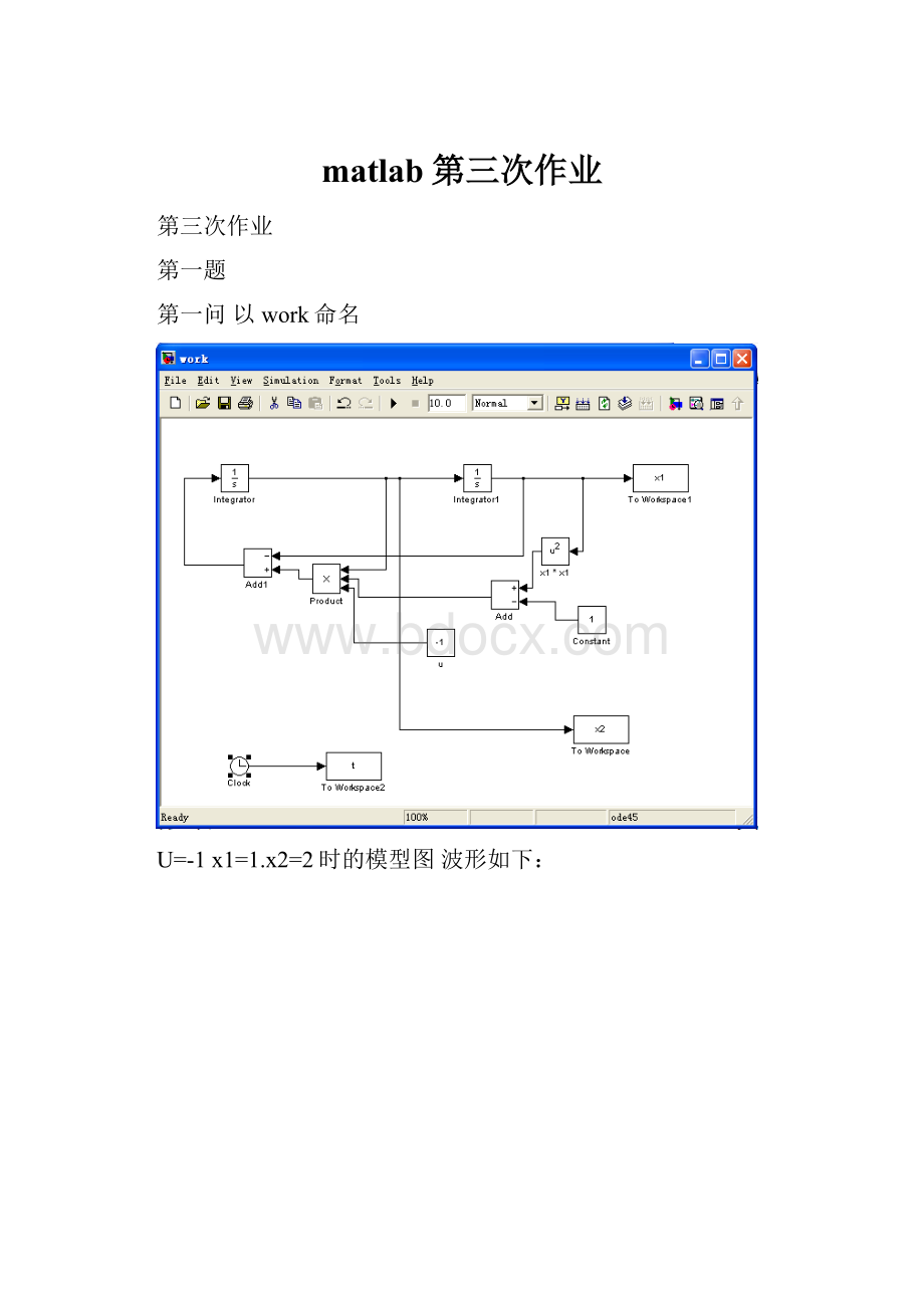
第一问以work命名

U=-1x1=1.x2=2时的模型图波形如下：

平面曲线

时间响应

U=2x1=-0.2x2=-0.7的模型图波形如下

平面曲线

时间响应

第二问

U=-1x1=1.x2=2时的模型图

XYGraph图如下

示波器图如下

U=2x1=-0.2x2=-0.7的模型图如下

XYGraph图如下

示波器图如下

二小题

[a,b,c,d]=linmod（'No21'）

Indlinmodat176

Inlinmodat54

a=

001.00000

0001.0000

0000

1.0000000

b=

Emptymatrix:

4-by-0

c=

Emptymatrix:

0-by-4

d=

[]

>>sys=ss（a,b,c,d）

a=

x1x2x3x4

x10010

x20001

x30000

x41000

b=

Emptymatrix:

4-by-0

c=

Emptymatrix:

0-by-4

d=

[]

Continuous-timemodel.

>>tf（sys）

Emptytransferfunction.

第二问

Matlab仿真图

将k21，k12，k23，k32，1、v1*wt均换成实数2得到新的matlab仿真图

[a,b,c,d]=linmod（'No22'）

Indlinmodat176

Inlinmodat54

a=

-2.00002.00000

2.0000-4.00002.0000

02.0000-2.0000

b=

01.0000

00

00

c=

000

000

1.000000

01.00000

001.0000

d=

10

00

00

00

00

>>sys=ss（a,b,c,d）

a=

x1x2x3

x1-220

x22-42

x302-2

b=

u1u2

x101

x200

x300

c=

x1x2x3

y1000

y2000

y3100

y4010

y5001

d=

u1u2

y110

y200

y300

y400

y500

Continuous-timemodel.

>>tf（sys）

Transferfunctionfrominput1tooutput...

#1:

1

#2:

0

#3:

0

#4:

0

#5:

0

Transferfunctionfrominput2tooutput...

#1:

0

#2:

0

s^2+6s+4

#3:

-------------------------------

s^3+8s^2+12s-1.223e-015

2s+4

#4:

-------------------------------

s^3+8s^2+12s-1.223e-015

4

#5:

-------------------------------

s^3+8s^2+12s-1.223e-015

第三小题

方法一：

方法二

第四小题

plot（tout,y）

>>legend（'cos','sin'）

状态曲线

Plot（tout，x）

legend（'x1','x2','x3','x4'）

plot（tout,y）

>>legend（'cos','sin'）

状态曲线

Plot（tout，x）

legend（'x1','x2','x3','x4'）

A=

2.2500-5.0000-1.2500-0.5000

2.2500-4.2500-1.2500-0.2500

0.2500-0.5000-1.2500-1.0000

1.2500-1.7500-0.2500-0.7500

>>B=[46;24;22;02]

B=

46

24

22

02

>>c=[1000;0100;0010;0001]

c=

1000

0100

0010

0001

>>d=[00;00;00;00]

d=

00

00

00

00

>>sys=ss（A,B,c,d）

a=

x1x2x3x4

x12.25-5-1.25-0.5

x22.25-4.25-1.25-0.25

x30.25-0.5-1.25-1

x41.25-1.75-0.25-0.75

b=

u1u2

x146

x224

x322

x402

c=

x1x2x3x4

y11000

y20100

y30010

y40001

d=

u1u2

y100

y200

y300

y400

Continuous-timemodel.

>>tf（sys）

Transferfunctionfrominput1tooutput...

4s^3+12.5s^2+15.75s+9

#1:

--------------------------------------

s^4+4s^3+6.25s^2+5.25s+2.25

2s^3+6s^2+8s+5.25

#2:

--------------------------------------

s^4+4s^3+6.25s^2+5.25s+2.25

2s^3+5.5s^2+4.75s+1.5

#3:

--------------------------------------

s^4+4s^3+6.25s^2+5.25s+2.25

s^2+3s+2.25

#4:

--------------------------------------

s^4+4s^3+6.25s^2+5.25s+2.25

Transferfunctionfrominput2tooutput...

6s^3+14s^2+14.5s+5.25

#1:

--------------------------------------

s^4+4s^3+6.25s^2+5.25s+2.25

4s^3+9.5s^2+10.75s+4.75

#2:

--------------------------------------

s^4+4s^3+6.25s^2+5.25s+2.25

2s^3+3s^2+s-0.25

#3:

--------------------------------------

s^4+4s^3+6.25s^2+5.25s+2.25

2s^3+6.5s^2+7.75s+3.75

#4:

--------------------------------------

s^4+4s^3+6.25s^2+5.25s+2.25

plot（tout,y）

>>legend（'cos','sin'）

plot（tout,x1）

legend（'x1'）

plot（tout,x2）

legend（'x2'）

plot（tout,x3）

legend（'x3'）

plot（tout,x4）

legend（'x4'）

第五小题

第二问

第二大题

第一小题

第二小题

Matlab仿真图

子系统封装图

第三大题

第一小题

阶跃响应图如下

第二小题

频率为20Hz时的电流曲线

频率为40Hz时的电流曲线

频率为60Hz时的电流曲线

第三小题

波形图