Multiple Linear Regression Model1.docx
《Multiple Linear Regression Model1.docx》由会员分享,可在线阅读,更多相关《Multiple Linear Regression Model1.docx(12页珍藏版)》请在冰豆网上搜索。
MultipleLinearRegressionModel1
MultipleLinearRegressionModel
Ⅰ.Introduction
ByusingRsoftwareestimationcanbeturnedintolinearregressionmodelofthenonlinearmodel,andtheparametersofthelinearregressionmodeltestoflinearconstraints.Thisexperimentonthegrossvalueofindustrialoutputandassetsandworkernumberoflinearityregressionanalysis.
Ⅱ.Caseintroduced
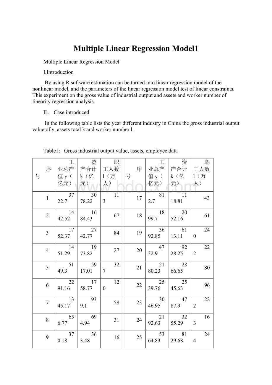
InthefollowingtableliststheyeardifferentindustryinChinathegrossindustrialoutputvalueofy,assetstotalkandworkernumberl.
Table1:
Grossindustrialoutputvalue,assets,employeedata
序号
工业总产值y(亿元)
资产合计k(亿元)
职工人数l(万人)
序号
工业总产值y(亿元)
资产合计k(亿元)
职工人数l(万人)
1
3722.7
3078.22
113
17
812.7
1118.81
43
2
1442.52
1684.43
67
18
1899.7
2052.16
61
3
1752.37
2742.77
84
19
3692.85
6113.11
240
4
1451.29
1973.82
27
20
4732.9
9228.25
222
5
5149.3
5917.01
327
21
2180.23
2866.65
80
6
2291.16
1758.77
120
22
2539.76
2545.63
96
7
1345.17
939.1
58
23
3046.95
4787.9
222
8
656.77
694.94
31
24
2192.63
3255.29
163
9
370.18
363.48
16
25
5364.83
8129.68
244
10
1590.36
2511.99
66
26
4834.68
5260.2
145
11
616.71
973.73
58
27
7549.58
7518.79
138
12
617.94
516.01
28
28
867.91
984.52
46
13
4429.19
3785.91
61
29
4611.39
18626.94
218
14
5749.02
8688.03
254
30
170.3
610.91
19
15
1781.37
2798.9
83
31
325.53
1523.19
45
16
1243.07
1808.44
33
Ⅲ.ModelBuilding
3.1.Model_1Setamodelfor
Step1:
Readthedata
>da=read.table("C:
/23/f.csv",sep=",")
>y=da[,2]
>k=da[,3]
>l=da[,4]
>win.graph(width=3.5,height=3.5,pointsize=8)
>plot(y,k)#plotthescatterofyandk
>plot(y,l)#plotthescatterofyandl
Step2:
PARAMETERESTIMATION
>m1=lm(y~k+l)
>summary(m1)
Call:
lm(formula=y~k+l)
Residuals:
Min1QMedian3QMax
-2113.0-472.9-232.7196.53928.2
Coefficients:
EstimateStd.ErrortvaluePr(>|t|)
(Intercept)588.61734339.389361.7340.09386.
k0.199260.081942.4320.02167*
l11.120213.622673.0700.00473**
---
Signif.codes:
0‘***’0.001‘**’0.01‘*’0.05‘.’0.1‘’1
Residualstandarderror:
1143on28degreesoffreedom
MultipleR-squared:
0.6715,AdjustedR-squared:
0.648
F-statistic:
28.62on2and28DF,p-value:
1.706e-07
Itisconcludedthatthefollowingregressionequation:
Analysisofvariance
>anova(m1)
AnalysisofVarianceTable
Response:
y
DfSumSqMeanSqFvaluePr(>F)
k1624666966246669647.80771.624e-07***
l112311730123117309.42250.004725**
Residuals28365854951306625
---
Signif.codes:
0‘***’0.001‘**’0.01‘*’0.05‘.’0.1‘’1
Residualanalysis
>re1=residuals(m1)
>plot(re1)
Step3:
Resultsanalysis
1.coefficientofdetermination
BecauseofR^2=0.6715,sothefittingeffectisnotgood
2.TESTSOFHYPOTHESES
Agivenlevelofsignificance:
>qf(0.975,2,27)
[1]4.242094
>qt(0.975,27)
[1]2.051831
F=28.62>F(2,27)=4.24
P=1.706e-07<0.05,Showthatk,lcombinedtohaveasignificantlinearimpactony.
T(k)=2.432〉t(27)=2.05;T(l)=3.070〉t(27)=2.05,Showthatk,lofyhassignificantlinearinfluence.
3.Accordingtotheresidualfigure,wecanfindthatasthedatasequence,residualobviousdeviationfromthemean,theincreasescope,showedthatpoorregressionresults.
4.Theregressionequationresidualanalysis
>plot(m1)
Fromtheaboveknowable,deviatingfromthefittinglinesituationisrelativelyserious,canalsobeconcludedthatthefittingeffectisnotgood.
3.2.Model2
Setamodelfor
Thelogarithmictransformation,
Canbeconvertedinto
Step1:
DATAPROCESSING
>y1=log(y)#takelogarithms
>k1=log(k)
>l1=log(l)
Table2:
data(ln)
Serialnumber
Grossvalueofindustrialoutput
lnY
Assetstotal
lnK
Theworkernumber
lnL
(亿元)
(亿元)
(万人)
1
8.222204
8.032107
4.727388
2
7.274147
7.429183
4.204693
3
7.468724
7.916724
4.430817
4
7.280208
7.587726
3.295837
5
8.546616
8.685587
5.78996
6
7.736814
7.47237
4.787492
7
7.204276
6.844922
4.060443
8
6.487334
6.543826
3.433987
9
5.913989
5.895724
2.772589
10
7.371716
7.828831
4.189655
11
6.424399
6.881134
4.060443
12
6.426391
6.246126
3.332205
13
8.395972
8.239042
4.110874
14
8.656785
9.069701
5.537334
15
7.485138
7.936982
4.418841
16
7.125339
7.50022
3.496508
17
6.700362
7.020021
3.7612
18
7.549451
7.626648
4.110874
19
8.214154
8.718191
5.480639
20
8.462293
9.130025
5.402677
21
7.687186
7.960899
4.382027
22
7.839825
7.842133
4.564348
23
8.021896
8.473847
5.402677
24
7.692857
8.088037
5.09375
25
8.58762
9.003277
5.497168
26
8.48357
8.567924
4.976734
27
8.929247
8.92516
4.927254
28
6.766088
6.892154
3.828641
29
8.436285
9.832364
5.384495
30
5.137562
6.41495
2.944439
31
5.785455
7.328562
3.806662
Step2:
Parameterestimation
>m2=lm(log(y)~log(k)+log(l))
>summary(m2)
Call:
lm(formula=log(y)~log(k)+log(l))
Residuals:
Min1QMedian3QMax
-1.20679-0.155170.031790.265320.73927
Coefficients:
EstimateStd.ErrortvaluePr(>|t|)
(Intercept)1.15400.72761.5860.12397
log(k)0.60920.17643.4540.00178**
log(l)0.36080.20161.7900.08432.
---
Signif.codes:
0‘***’0.001‘**’0.01‘*’0.05‘.’0.1‘’1
Residualstandarderror:
0.4255on28degreesoffreedom
MultipleR-squared:
0.8099,AdjustedR-squared:
0.7963
F-statistic:
59.66on2and28DF,p-value:
8.035e-11
Itisconcludedthatthefollowingregressionequation:
(exp(1.1540)=3.170851)
Analysisofvariance
>anova(m2)
AnalysisofVarianceTable
Response:
log(y)
DfSumSqMeanSqFvaluePr(>F)
log(k)121.024921.0249116.10691.805e-11***
log(l)10.58000.58003.20320.08432.
Residuals285.07030.1811
---
Signif.codes:
0‘***’0.001‘**’0.01‘*’0.05‘.’0.1‘’1
Residualanalysis
>re2=residuals(m2)
>plot(re2)
>
Step3:
Resultsanalysis
2.coefficientofdetermination
:
BecauseofR^2=0.8099,Sothefittingeffectisbetterthanmodel1.
3.TESTSOFHYPOTHESES
Agivenlevelofsignificanceis5%,
>qf(0.975,2,27)
[1]4.242094
>qt(0.975,27)
[1]2.051831
F=59.66>F(2,27)=4.24
P=8.035e-11<0.05,ShowthatLNK,LNLcombinedtohaveasignificantlinearimpactonlny
。
T(lnk)=3.454>2.05,T(lnl)=1.790<2.05,LNKparametersthroughthetestofsignificanceofvariables;ButtheparametersoftheLNLfailedtheinspection.
Ifagiven10%significancelevel
>qt(0.95,27)
[1]1.703288
T(lnk)=3.454>1.70;T(lnl)=1.790>1.70,SotheLNK,LNLparametersthroughthetestofsignificanceofvariables.
3.Accordingtotheresidualfigure,wecanfindthatinadditiontothethreeabnormalpointsafter,evenlydistributedaroundthezeroresidual,andvolatility,within0.5regressionresultisgood.
4.Theregressionequationresidualfigure
>plot(m2)
 升级会员
升级会员 