机械原理使用矩阵法对图所示机构进行运动分析.docx
《机械原理使用矩阵法对图所示机构进行运动分析.docx》由会员分享,可在线阅读,更多相关《机械原理使用矩阵法对图所示机构进行运动分析.docx(16页珍藏版)》请在冰豆网上搜索。
机械原理使用矩阵法对图所示机构进行运动分析
机械原理使用矩阵法对图所示机构进行运动分析
机械原理作业
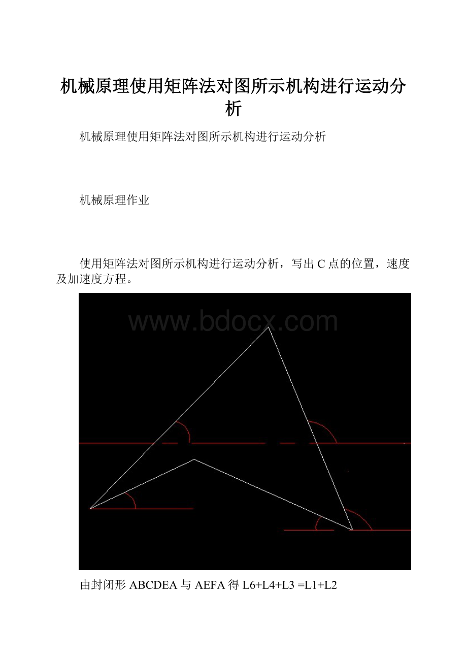
使用矩阵法对图所示机构进行运动分析,写出C点的位置,速度及加速度方程。
由封闭形ABCDEA与AEFA得L6+L4+L3=L1+L2
L1’=L6+L4’
(1)位置分析
机构的封闭矢量方程式写成在两坐标上的投影表达式:
由以上方程求出θ2θ3θ4L1’
利用非线性超越方程组牛顿—辛普森求解方法原理:
设:
f1(θ2θ3θ4L1’)=L2cosθ2-L3cosθ3+L4cosθ4-L1cosθ1-L6=0
f2(θ2θ3θ4L1’)=L2sinθ2-L3sinθ3+L4sinθ4-L1θ1=0
f3(θ2θ3θ4L1’)=-L4’θ4+L1’cosθ1-L6=0
f3(θ2θ3θ4L1’)=-L4’sinθ4+L1’sinθ1=0
J=[-x(6)*sin(theta2)x(7)*sin(theta3)-x(8)*sin(theta4)0;
x(6)*cos(theta2)-x(7)*cos(theta3)x(8)*cos(theta4)0;
00x(10)*sin(theta4)cos(x
(1));
00-x(10)*cos(theta4)sin(x
(1))]
(2)速度分析
对位置方程组求导:
-L2*w2*sinθ2+L3*w3*sinθ3-L4*w4*sinθ4+L1*w1sinθ1=0
L2*w2*cosθ2-L3*w3*cosθ3+L4*w4*cosθ4-L1*w1cosθ1=0
L4’*w4*sinθ4+L1’’*cosθ1-L1’*w1*sinθ1=0
-L4’*w4*cosθ4+L1’’*sinθ1+L1’*w1*cosθ1=0
可得w2、w3、w4、L1’’。
上式表达为矩阵形式:
-L2*sinθ2L3*sinθ3-L4*sinθ40w2-L1*sinθ1
L2*cosθ2-L3*cosθ3L4*cosθ40w3L1*cosθ1
00L4’*sinθ4cosθ1w4L1’*sinθ1
00-L4’*cosθ4sinθ1L1’’-L1’*cosθ1
(3)加速度分析
将速度方程求导,可得加速度关系式
≈
-L2*w2*cosθ2L3*w3*cosθ3-L4*w4*cosθ40w2
-L2*w2*sinθ2L3*w3*sinθ3-L4*w4*sinθ40w3
00L4’*w4*cosθ4-w1*sinθ1w4
00-L4’*w4*sinθ4w1*cosθ1L1’’
-L2*sinθ2L3*sinθ3-L4*sinθ40α2
+L2*cosθ2-L3*cosθ3L4*cosθ40α3
00L4’*sinθ4cosθ1α4
00-L4’*cosθ4sinθ1L1’’’
-L1*w1*cosθ1
w1-L1*w1*sinθ1
L1’’*sinθ1+L1’*w1*cosθ1
-L1’’*cosθ1+L1’*w1*sinθ1
用MATLAB编程运行
(1)对位置方程进行求解
在此机构中,因为FE杆是定值60mm、AE为定值70mm,当DE杆垂直于BF杆时,θ1达到最大值,即sinθ1(max)=EF/AE=60/70,可得θ1(max)=58.99*pi/180。
编制程序如下:
functiony=rrrposi(x)
%
%ScriptusedtoimplementNewton-Raphonmechodfor
%solvingnonlinearpositionofRRRbargroup
%
%Inputparameters
%
%x
(1)=theta-1
%x
(2)=theta-2guessvalue
%x(3)=theta-3guessvalue
%x(4)=theta-4guessvalue
%x(5)=r1
%x(6)=r2
%x(7)=r3
%x(8)=r4
%x(9)=r5
%x(10)=r6
%x(11)=r7guessvalue
%
%Outputparamenters
%
%y
(1)=theta-2
%y
(2)=theta-3
%y(3)=theta-4
%y(4)=r7
%
theta2=x
(2);
theta3=x(3);
theta4=x(4);
r8=x(11)
%
epsilon=1.0E-6;
%
f=[-x(5)*cos(x
(1))+x(6)*cos(theta2)-x(7)*cos(theta3)+x(8)*cos(theta4)-x(9);
-x(5)*sin(x
(1))+x(6)*sin(theta2)-x(7)*sin(theta3)+x(8)*sin(theta4);
-x(9)-x(10)*cos(theta4)+r8*cos(x
(1));
-x(10)*sin(theta4)+r8*sin(x
(1))];
%
whilenorm(f)>epsilon
J=[-x(6)*sin(theta2)x(7)*sin(theta3)-x(8)*sin(theta4)0;
x(6)*cos(theta2)-x(7)*cos(theta3)x(8)*cos(theta4)0;
00x(10)*sin(theta4)cos(x
(1));
00-x(10)*cos(theta4)sin(x
(1))];
dth=inv(J)*(-1.0*f);
theta2=theta2+dth
(1);
theta3=theta3+dth
(2);
theta4=theta4+dth(3);
r8=r8+dth(4);
%
f=[-x(5)*cos(x
(1))+x(6)*cos(theta2)-x(7)*cos(theta3)+x(8)*cos(theta4)-x(9);
-x(5)*sin(x
(1))+x(6)*sin(theta2)-x(7)*sin(theta3)+x(8)*sin(theta4);
-x(9)-x(10)*cos(theta4)+r8*cos(x
(1));
-x(10)*sin(theta4)+r8*sin(x
(1))];
norm(f);
end;
y
(1)=theta2;
y
(2)=theta3;
y(3)=theta4;
y(4)=r8;
>>x1=linspace(43*pi/180,58*pi/180,15);
x=zeros(length(x1),11);
forn=1:
15
x(n,:
)=[x1(:
n)30*pi/180160*pi/180120*pi/18040507535706066];
end;
p=zeros(length(x1),4);
fork=1:
15
y=rrrposi0(x(k,:
));
p(k,:
)=y;
end;
p
r8=66
p=
0.68382.59271.670687.5390
0.67252.61091.715985.3559
0.66142.63001.761783.1049
0.65042.64981.808080.7822
0.63942.67051.855178.3827
0.62852.69201.903075.9002
0.61762.71461.951873.3264
0.60662.73822.001770.6505
0.59532.76312.053067.8576
0.58362.78952.106164.9269
0.57132.81782.161461.8275
0.55792.84842.219758.5110
0.54272.88242.282654.8943
0.52412.92202.352650.8105
0.49762.97272.437345.8116
结果依次表示为:
θ2*pi/180、θ3*pi/180、θ4*pi/180、L1’的值。
(2)速度方程求解:
编程如下:
functiony=rrrvel(x)
%
%Inputparameters
%
%x
(1)=theta-1
%x
(2)=theta-2
%x(3)=theta-3
%x(4)=theta-4
%x(5)=dtheta-1
%x(6)=r1
%x(7)=r2
%x(8)=r3
%x(9)=r4
%x(10)=r5
%x(11)=r6
%
%Outputparameters
%
%y
(1)=dtheta-2
%y
(2)=dtheta-3
%y(3)=dtheta-4
%y(4)=dr1
%
A=[-x(8)*sin(x
(2))x(9)*sin(x(3))-x(10)*sin(x(4))0;
x(8)*cos(x
(2))-x(9)*cos(x(3))x(10)*cos(x(9))0;
00x(11)*sin(x(4))cos(x
(1));
00-x(11)*cos(x(4))sin(x
(1))];
B=[-x(7)*sin(x
(1));x(7)*cos(x
(1));x(6)*sin(x
(1));-x(6)*cos(x
(1))]*x(5);
y=inv(A)*B;
输入数据
>>x2=[x1'p(:
1)p(:
2)p(:
3)10*ones(15,1)p(:
4)40*ones(15,1)50*ones(15,1)75*ones(15,1)35*ones(15,1)60*ones(15,1)];
q=zeros(4,15);
form=1:
15
y2=rrrvel(x2(m,:
));
q(:
m)=y2;
end;
q
q=
1.0e+003*
Columns1through9
-0.0156-0.0158-0.0161-0.0164-0.0166-0.0170-0.0173-0.0177-0.0182
0.00190.00190.00190.00180.00180.00180.00170.00160.0015
0.02410.02430.02460.02500.02540.02580.02640.02700.0279
-1.1499-1.1853-1.2225-1.2621-1.3047-1.3511-1.4025-1.4607-1.5282
Columns10through15
-0.0188-0.0196-0.0208-0.0227-0.0261-0.0352
0.00130.00120.00100.00080.00070.0009
0.02890.03030.03220.03520.04030.0526
-1.6090-1.7101-1.8440-2.0378-2.3631-3.1197
结果纵向依次为:
w2、w3、w4、L1’’(v)的值。
(3)加速度的分析
编程如下
functiony=rrra(x)
%
%inputparameters
%
%x
(1)=th1
%x
(2)=th2
%x(3)=th3
%x(4)=th4
%x(5)=dth1
%x(6)=dth2
%x(7)=dth3
%x(8)=dth4
%x(9)=r1
%x(10)=r2
%x(11)=r3
%x(12)=r4
%x(13)=r5
%x(14)=r6
%x(15)=r7
%
%y
(1)=ddth2
%y
(2)=ddth3
%y(3)=ddth4
%y(4)=dr1
%
A=[-x(11)*sin(x
(2))x(12)*sin(x(3))-x(13)*sin(x(4))0;
x(11)*cos(x
(2))-x(12)*cos(x(3))x(13)*cos(x(4))0;
00x(14)*sin(x(4))cos(x
(1));
00-x(14)*cos(x(4))sin(x
(1))];
B=[-x(11)*x(6)*cos(x
(2))x(12)*x(7)*cos(x(3))-x(13)*x(8)*cos(x(4))0;
-x(11)*x(6)*sin(x
(2))x(12)*x(7)*sin(x(3))-x(13)*x(8)*sin(x(4))0;
00x(14)*x(8)*cos(x(4))-x(5)*sin(x
(1));
00x(14)*x(8)*sin(x(4))x(5)*cos(x
(1))];
C=[x(6);x(7);x(8);x(9)];
D=[-x(9)*x(5)*cos(x
(1));-x(9)*x(5)*sin(x
(1));x(9)*sin(x
(1))+x(9)*x(5)*cos(x
(1));-x(9)*cos(x
(1))+x(9)*x(5)*sin(x
(1))];
y=inv(A)*D*x(5)-inv(A)*B*C;
输入数据
>>x3=[x1'p(:
1)p(:
2)p(:
3)10*ones(15,1)q(1,:
)'q(2,:
)'q(3,:
)'q(4,:
)'40*ones(15,1)50*ones(15,1)75*ones(15,1)35*ones(15,1)p(:
4)60*ones(15,1)];
f=zeros(4,15);
form=1:
15
y3=rrra(x3(m,:
));
f(:
m)=y3;
end;
f
f=
1.0e+005*
Columns1through12
-0.0068-0.0071-0.0074-0.0078-0.0083-0.0089-0.0095-0.0104-0.0115-0.0129-0.0149-0.0180
0.02090.02170.02250.02340.02440.02550.02680.02840.03030.03270.03590.0408
0.00330.00350.00370.00390.00420.00460.00510.00560.00640.00750.00910.0119
-1.6862-1.7217-1.7602-1.8025-1.8498-1.9039-1.9672-2.0434-2.1384-2.2625-2.4343-2.6931
Columns13through15
-0.0233-0.0351-0.0817
0.04890.06620.1309
0.01740.03120.0943
-3.1360-4.0878-7.5791
结果为:
a2、a3、a4、L1’的加速度。
位置,速度,加速度数据总表:
θ1
θ2
θ3
θ4
L1’
w2
W3
W4
v(L1’)
α2
α3
α4
a(L1’)
rad
mm
rad/s
rad/s
rad/s
mm/s
rad/sˇ2
mm/sˇ2
0.75049
0.68378
2.5927
1.6706
87.539
-0.0156
0.0019
0.0241
-1.1499
-0.0068
0.0209
0.0033
-1.6862
0.76919
0.6725
2.6109
1.7159
85.356
-0.0158
0.0019
0.0243
-1.1853
-0.0071
0.0217
0.0035
-1.7217
0.78789
0.66138
2.63
1.7617
83.105
-0.0161
0.0019
0.0246
-1.2225
-0.0074
0.0225
0.0037
-1.7602
0.80659
0.65036
2.6498
1.808
80.782
-0.0164
0.0018
0.025
-1.2621
-0.0078
0.0234
0.0039
-1.8025
0.82529
0.63943
2.6705
1.8551
78.383
-0.0166
0.0018
0.0254
-1.3047
-0.0083
0.0244
0.0042
-1.8498
0.84399
0.62853
2.692
1.903
75.9
-0.017
0.0018
0.0258
-1.3511
-0.0089
0.0255
0.0046
-1.9039
0.86269
0.6176
2.7146
1.9518
73.326
-0.0173
0.0017
0.0264
-1.4025
-0.0095
0.0268
0.0051
-1.9672
0.88139
0.60656
2.7382
2.0017
70.651
-0.0177
0.0016
0.027
-1.4607
-0.0104
0.0284
0.0056
-2.0434
0.90009
0.59529
2.7631
2.053
67.858
-0.0182
0.0015
0.0279
-1.5282
-0.0115
0.0303
0.0064
-2.1384
0.91879
0.58362
2.7895
2.1061
64.927
-0.0188
0.0013
0.0289
-1.609
-0.0129
0.0327
0.0075
-2.2625
0.93749
0.5713
2.8178
2.1614
61.827
-0.0196
0.0012
0.0303
-1.7101
0.0149
0.0359
0.0091
-2.4343
0.95619
0.55791
2.8484
2.2197
58.511
-0.0208
0.001
0.0322
-1.844
-0.018
0.0408
0.0119
-2.6931
0.97489
0.54271
2.8824
2.2826
54.894
-0.0277
0.0008
0.0352
-2.0378
-0.0233
0.0489
0.0174
-3.316
0.99359
0.52411
2.922
2.3526
50.811
-0.0261
0.0007
0.0403
0.0526
-0.0351
0.0662
0.0312
-4.0878
1.0123
0.49762
2.9727
2.4373
45.812
-0.0352
0.0009
0.0526
-3.1197
-0.0817
0.1309
0.0943
-7.5791
输出图像如下:
>>plot(x1,p(1,:
),'--',x1,p(2,:
),':
',x1,p(3,:
),'*')
即θ2、θ3、θ4关于θ1的函数图。
>>plot(x1,p(4,:
))
即L1’关于θ1的函数图。
>>plot(x1,q(1,:
),'--',x1,q(2,:
),':
',x1,q(3,:
),'*')
即w2、w3、w4关于θ1的函数图。
>>plot(x1,f(4,:
))
即杆L1’的速度关于θ1的函数图。
>>plot(x1,f(1,:
),'p',x1,f(2,:
),x1,f(3,:
),'*')
即α2、α3、α4关于θ1的函数图。
>>plot(x1,f(4,:
))
即杆L1’的加速度关于θ1的函数图。
 升级会员
升级会员 