数字信号处理matlab作业.docx
《数字信号处理matlab作业.docx》由会员分享,可在线阅读,更多相关《数字信号处理matlab作业.docx(24页珍藏版)》请在冰豆网上搜索。
数字信号处理matlab作业
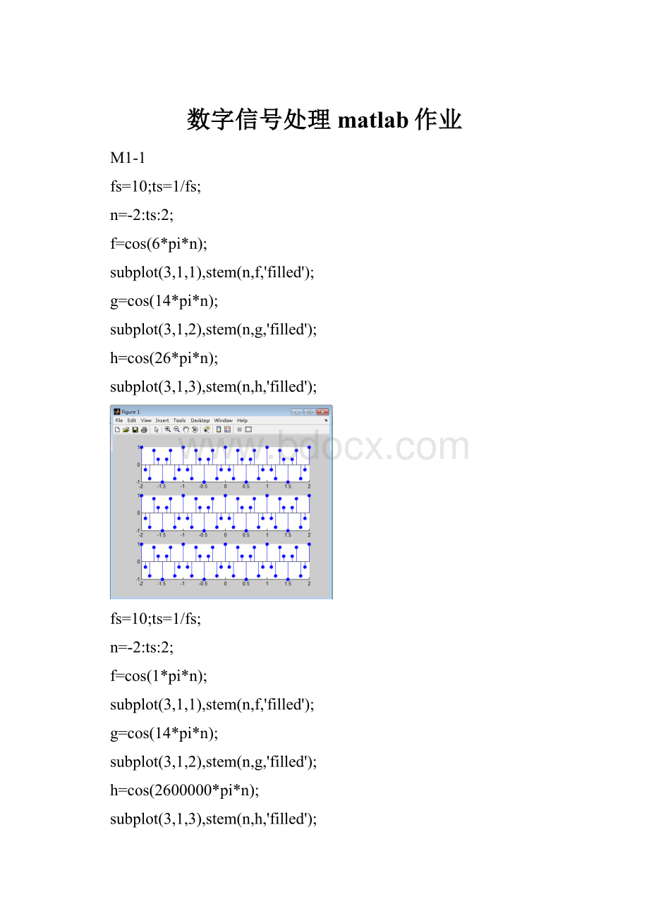
M1-1
fs=10;ts=1/fs;
n=-2:
ts:
2;
f=cos(6*pi*n);
subplot(3,1,1),stem(n,f,'filled');
g=cos(14*pi*n);
subplot(3,1,2),stem(n,g,'filled');
h=cos(26*pi*n);
subplot(3,1,3),stem(n,h,'filled');
fs=10;ts=1/fs;
n=-2:
ts:
2;
f=cos(1*pi*n);
subplot(3,1,1),stem(n,f,'filled');
g=cos(14*pi*n);
subplot(3,1,2),stem(n,g,'filled');
h=cos(2600000*pi*n);
subplot(3,1,3),stem(n,h,'filled');
M2-1
(1)x=[1-3420-2];h=[301-121];
L=length(x)+length(h)-1;
XE=fft(x,L);
HE=fft(h,L);
y1=ifft(XE.*HE);
y=[10-1010];g=[1392781243]
M=length(y)+length(g)-1;
YE=fft(y,M);
GE=fft(g,M);
y2=ifft(YE.*GE);
a=0:
L-1;
subplot(2,1,1);
stem(a,real(y1));
b=0:
M-1;
subplot(2,1,2);
stem(b,real(y2));
M2-2
N=10;
k=0:
N-1;
f=cos(pi*k/20);
F=fft(f);
plot(k/10,abs(F),'o');
holdon
set(gca,'xtick',[0,0.25,0.5,0.75,1]);
set(gca,'ytick',[0,2,4,6,8]);
gridon
holdoff
M2-3
N=input('lenthofsignal:
N=');
M=input('pointsofDFT:
M=');
k=0:
N-1;
f=cos(2*pi*100*k/600)+cos(2*pi*150*k/600);%0.15*
w=hamming(length(f));
f=f*w;%加hamming窗
F=fft(f,M);
L=0:
(M-1);
plot(L/M,abs(F))
gridon;
xlabel('Normalizedfrequency');
ylabel('Magnitude');
M2-4
M=4;N=64;
n=-(N-1)/2:
(N-1)/2;
x=cos(2*pi*n/15)+0.75*cos(2.3*pi*n/15);
X=fft(x,N);
subplot(2,1,1);stem(n,fftshift(x));
ylabel('x[n]');xlabel('Timen');
subplot(2,1,2);
stem(omega,real(fftshift(X)));
ylabel('X[k]');
xlabel('Frequency(rad)');
hold;
M2-5
w=linspace(0,10,1024);
plot(w,2./(w.^2+1));
%samplingpointsandfrequency(rad/s)
N=input('抽样点数=');
Ws=input('抽样角频率=');
Ts=2*pi/Ws;
%computethesamplingpoints
k=0:
N/2;
t=k*Ts;
f1=exp(-3*t);
f1(N/2+1)=2*f1(N/2+1);
f2=f1(2:
N/2);
f=[f1fliplr(f2)];
F=Ts*real(fft(f));
w=k*Ws/N;
w1=linspace(0,Ws/2,512);
plot(w1,2./(w1.^2+1),w,F(1:
N/2+1),'r');
axis([01002.2]);
xlabel('频率(秒/弧度)');
ylabel('幅度');
z=['N='num2str(N)'Ws='num2str(Ws)'的结果'];
legend('理论值',z);
title('exp(-|t|)的谱');
M4-1
wp=10;ws=2;Ap=1;As=40;
[N,Wc]=cheb1ord(wp,ws,Ap,As,'s');
[num,den]=cheby1(N,Ap,Wc,'s');
disp('LP分子多项式');
fprintf('%.4e\n',num);
disp('LP分母多项式');
fprintf('%.4e\n',den);
[numt,dent]=lp2hp(num,den,1);
disp('HP分子多项式');
fprintf('%.4e\n',numt);
disp('LP分母多项式');
fprintf('%.4e\n',dent);
M4-2
wp=1;ws=3.3182;Ap=1;As=32;
w0=sqrt(48);B=2;
[N,Wc]=buttord(wp,ws,Ap,As,'s');
[num,den]=butter(N,Wc,'s');
[numt,dent]=lp2bp(num,den,w0,B);
w=linspace(2,12,1000);
h=freqs(numt,dent,w);
plot(w,20*log10(abs(h)));grid;
xlabel('Frequencyinrad/s');
ylabel('GainindB');
M4-3
wp=1;ws=3.3182;Ap=1;As=32;
w0=sqrt(48);B=2;
[N,Wc]=ellipord(wp,ws,Ap,As,'s');
[num,den]=ellip(N,Ap,As,Wc,'s');
[numt,dent]=lp2bp(num,den,w0,B);
w=linspace(2,12,1000);
h=freqs(numt,dent,w);
plot(w,20*log10(abs(h)));grid;
xlabel('Frequencyinrad/s');
ylabel('GainindB');
M4-4
Ap=1;As=10;wp1=6;wp2=13;ws1=9;ws2=11;
B=ws2-ws1;w0=sqrt(ws1*ws2);
wLp1=B*wp1/(w0*w0-wp1*wp1);
wLp2=B*wp2/(w0*w0-wp2*wp2);
wLp=max(abs(wLp1),abs(wLp2));
[N,wc]=ellipord(wp,ws,Ap,As,'s');
[num,den]=ellip(N,Ap,As,Wc,'s');
[numt,dent]=lp2bs(num,den,w0,B);
w=linspace(5,35,1000);
h=freqs(numt,dent,w);
plot(w,20*log10(abs(h)));
w=[wp1ws1ws2wp2];
set(gca,'xtick',w);grid;
h=freqs(numt,dent,w);grid;
h=freqs(numt,dent,w);A=-20*log10(abs(h))
M4-5
Wp=0.1*pi;Ws=0.4*pi;Ap=1;As=25;
Fs=1;
wp=Wp*Fs;ws=Ws*Fs;
N=cheb2ord(wp,ws,Ap,As,'s');
wc=wp/(10^(0.1*Ap)-1)^(1/2/N);
[numa,dena]=cheby2(N,As,wc,'s');
[numd,dend]=impinvar(numa,dena,Fs);
w=linspace(0,pi,512);
h=freqz(numd,dend,w);
norm=max(abs(h));
numd=numd/norm;
plot(w*pi,20*log10(abs(h)/norm))
w=[WpWs]
h=freqz(numd,dend,w);
fprintf('Ap=%.4f\n',-20*log10(abs(h
(1))));
fprintf('Ap=%.4f\n',-20*log10(abs(h
(2))));
M4-6
M4-7
Wp=0.2*pi;Ws=0.4*pi;Ap=1;As=15;
Fs=1;
wp=Wp*Fs;ws=Ws*Fs;
N=cheb1ord(wp,ws,Ap,As,'s');
wc=wp/(10^(0.1*Ap)-1)^(1/2/N);
[numa,dena]=cheby1(N,Ap,wc,'s');
[numd,dend]=impinvar(numa,dena,Fs);
w=linspace(0,pi,512);
h=freqz(numd,dend,w);
norm=max(abs(h));
numd=numd/norm;
plot(w*pi,20*log10(abs(h)/norm))
w=[WpWs]
h=freqz(numd,dend,w);
fprintf('Ap=%.4f\n',-20*log10(abs(h
(1))));
fprintf('Ap=%.4f\n',-20*log10(abs(h
(2))));
M4-8
Wp=4*pi/44.1;Ws=20*pi/44.1;Ap=0.5;As=50;
Fs=44100;
wp=Wp*Fs;ws=Ws*Fs;
N=buttord(wp,ws,Ap,As,'s');
wc=wp/(10^(0.1*Ap)-1)^(1/N/2);
[numa,dena]=butter(N,wc,'s');
[numd,dend]=impinvar(numa,dena,Fs);
w=linspace(0,pi,1024);
h=freqz(numd,dend,w);
norm=max(abs(h));
numd=numd/norm;
plot(w/pi,20*log10(abs(h/norm)));
xlabel('f');
ylabel('Gain');
w=[WpWs];
h=freqz(numd,dend,w);
fprintf('Ap=%.4f\n',-20*log10(abs(h
(1))));
fprintf('As=%.4f\n',-20*log10(abs(h
(2))));
Wp=4*pi/44.1;Ws=20*pi/44.1;Ap=0.5;As=50;
T=2;Fs=1/T;
wp=2*tan(Wp/2)/T;ws=2*tan(Ws/2)/T;
[N,wc]=buttord(wp,ws,Ap,As,'s');
wc=wp/(10^(0.1*Ap)-1)^(1/N/2);
[numa,dena]=butter(N,wc,'s');
[numd,dend]=bilinear(numa,dena,Fs);
w=linspace(0,pi,1024);
h=freqz(numd,dend,w);
plot(w/pi,20*log10(abs(h)));
axis([01-500]);
xlabel('f');
ylabel('Gain');
w=[WpWs];
h=freqz(numd,dend,w);
fprintf('Ap=%.4f\n',-20*log10(abs(h
(1))));
fprintf('As=%.4f\n',-20*log10(abs(h
(2))));
M4-9
Wp=0.8*pi;Ws=0.6*pi;Ap=0.5;As=30;
T=2;Fs=1/T;
wp=2*tan(Wp/2)/T;ws=2*tan(Ws/2)/T;
[N,wc]=buttord(wp,ws,Ap,As,'s');
wc=wp/(10^(0.1*Ap)-1)^(1/N/2);
[numa,dena]=butter(N,wc,'s');
[numt,dent]=lp2hp(numa,dena,1);
[numd,dend]=bilinear(numt,dent,Fs);
w=linspace(0,pi,1024);
h=freqz(numd,dend,w);
plot(w/pi,20*log10(abs(h)));
axis([01-500]);
xlabel('f');
ylabel('Gain');
w=[WpWs];
h=freqz(numd,dend,w);
fprintf('Ap=%.4f\n',-20*log10(abs(h
(1))));
fprintf('As=%.4f\n',-20*log10(abs(h
(2))));
M5-1
functionFIR_LP
clear
clc
wp=0.2*pi;ws=0.3*pi;
tr_width=ws-wp;
N=ceil(6.6*pi/tr_width)+1;
n=[0:
1:
N-1];
wc=(ws+wp)/2;%理想LPF截止频
hd=ideal_lp(wc,N);%理想低通滤波器计算,hd=0-(N-1)之间的理想脉冲响应,wc=截止频率(弧度),N=理想滤波器的长度
wd1=hanning(N)';b1=hd.*wd1;
wd2=hamming(N)';b2=hd.*wd2;
wd3=blackman(N)';b3=hd.*wd3;
wd4=kaiser(N)';b4=hd.*wd4;
[db1,mag1,pha1,w]=freqz_m(b1,1);%汉宁窗
delta_w=2*pi/1000;
rp1=-(min(db1(1:
1:
wp/delta_w+1)));%实际带通波动
rp1
as1=-round(max(db1(ws/delta_w+1:
1:
501)));%最小带阻衰减
as1
[db2,mag2,pha2,w]=freqz_m(b2,1);%海明窗
delta_w=2*pi/1000;
rp2=-(min(db2(1:
1:
wp/delta_w+1)));%实际带通波动
rp2
as2=-round(max(db2(ws/delta_w+1:
1:
501)));%最小带阻衰减
as2
[db3,mag3,pha3,w]=freqz_m(b3,1);%blackman
delta_w=2*pi/1000;
rp3=-(min(db3(1:
1:
wp/delta_w+1)));%实际带通波动
rp3
as3=-round(max(db3(ws/delta_w+1:
1:
501)));%最小带阻衰减
as3
[db4,mag4,pha4,w]=freqz_m(b4,1);%kaiser
delta_w=2*pi/1000;
rp4=-(min(db4(1:
1:
wp/delta_w+1)));%实际带通波动
rp4
as4=-round(max(db4(ws/delta_w+1:
1:
501)));%最小带阻衰减
as4
figure
(1)
stem(n,hd);
title('理想脉冲响应')
axis([0N-1-0.10.3]);xlabel('n');ylabel('hd(n)');
figure
(2)
subplot(2,2,1)
plot(w,mag1,':
b')
legend('汉宁窗低通滤波器')
subplot(2,2,2)
plot(w,mag2,'-.g')
legend('海明窗低通滤波器')
subplot(2,2,3)
plot(w,mag3,'--r')
legend('布来克曼窗低通滤波器')
subplot(2,2,4)
plot(w,mag4,'-c')
legend('凯泽窗低通滤波器')
figure(3)
plot(w,mag1,':
b',w,mag2,'-.g',w,mag3,'--r',w,mag4,'-c')
legend('汉宁窗低通滤波器','海明窗低通滤波器','布来克曼窗低通滤波器','凯泽窗低通滤波器')
figure(4)
plot(w/pi,20*log10(mag1),':
b',w/pi,20*log10(mag2),'-.g',w/pi,20*log10(mag3),'--r',w/pi,20*log10(mag4),'-c')
legend('汉宁窗幅度响应(dB)','海明窗幅度响应(dB)','布来克曼窗幅度响应(dB)','凯泽窗幅度响应(dB)')
figure(5)
plot(n,b1,':
b',n,b2,'-.g',n,b3,'--r',n,b4,'-c')
legend('汉宁窗h(n)','海明窗h(n)','布来克曼窗h(n)','凯泽窗h(n)')
M5-2
Wp=0.6*pi;Ws=0.4*pi;Ap=1;As=45;
N=ceil(7*pi/(Wp-Ws));
N=mod(N+1,2)+N;
M=N-1;
w=hamming(N)';
Wc=(Wp+Ws)/2;
k=0:
M;
hd=-(Wc/pi)*sinc(Wc*(k-0.5*M)/pi);
hd(0.5*M+1)=hd(0.5*M+1)+1;
h=hd.*w;
omega=linspace(0,pi,512);
mag=freqz(h,[1],omega);
plot(omega/pi,20*log10(abs(mag)));
M5-4
N=40;
alfa=(40-1)/2;
k=0:
N-1;
w1=(2*pi/N)*k;
T1=0.109021;T2=0.59417456;
hrs=[zeros(1,5),T1,T2,ones(1,7),T2,T1,zeros(1,9),T1,T2,ones(1,7),T2,T1,zeros(1,4)];
hdr=[0,0,1,1,0,0];wd1=[0,0.2,0.35,0.65,0.8,1];
k1=0:
floor((N-1)/2);k2=floor((N-1)/2)+1:
N-1;
angH=[-alfa*(2*pi)/N*k1,alfa*(2*pi/N*(N-k2))];
H=hrs.*exp(j*angH);
h=real(ifft(H));
[db,mag,pha,grd,w]=freqz_m(h,1);
[Hr,ww,a,L]=Hr_Type2(h);
figure
(1)
subplot(2,2,1)
plot(w1(1:
21)/pi,hrs(1:
21),'o',wd1,hdr)
axis([0,1,-0.1,1.1]);
title('带通:
N=40,T1=0.109021,T2=0.59417456')
ylabel('Hr(k)');
set(gca,'XTickMode','manual','XTick',[0,0.2,0.35,0.65,0.8,1])
set(gca,'YTickMode','manual','YTick',[0,0.059,0.109,1]);
grid%绘制带网格的图像
subplot(2,2,2);
stem(k,h);
axis([-1,N,-0.4,0.4])
title('脉冲响应');ylabel('h(n)');text(N+1,-0.4,'n')
subplot(2,2,3);plot(ww/pi,Hr,w1(1:
21)/pi,hrs(1:
21),'o');
axis([0,1,-0.1,1.1]);title('振幅响应')
xlabel('频率(单位:
pi)');ylabel('Hr(w)')
set(gca,'XTickMode','manual','XTick',[0,0.2,0.35,0.65,0.8,1]);
set(gca,'YTickMode','manual','YTick',[0,0.059,0.109,1]);
grid
subplot(2,2,4);plot(w/pi,db);axis([0,1,-100,10]);
grid
title('幅度响应');xlabel('频率(单位:
pi)');ylabel('分贝')
set(gca,'XTickMode','manual','XTick',[0,0.2,0.35,0.65,0.8,1])
set(gca,'YTickMode','manual','YTick',[-60;0]);
set(gca,'YTickLabelMode','manual','YTickLabels',[60;0]);
[s,fs,nbits]=wavread('sj.wav');%信号de取样频率为44100HZ
x=s(:
1);
sound(x,fs);
L=length(x);
f=fs*(0:
L-1)/L;
t=0:
1/fs:
(L-1)/fs;%将所加噪声信号的点数调整到与原始信号相同
%Au=1
d=0.03*abs(max(x))*[cos(2*pi*22000*t)]';%噪声为500和3300Hz的余弦信号
%dz=cos(0.5*pi*fs*t)';%载波
dz=[cos(2*pi*11025*t)]';
xd=x.*dz;
xz=xd+d;
sound(xz,fs);%播放加噪声后的语音信号
X=fft(x);%求信号的频谱
XD=fft(xd);%信号调制后的频谱
XZ=fft(xz);
figure
(2)
subplot(3,1,1);plot(t,x)
title('未加噪的信号');xlabel('times');ylabel('幅度');
subplot(3,1,2);plot(t,xd)
title('调制后的信号');xlabel('times');ylabel('幅度');
subplot(3,1,3);plot(t,xz)
title('调制加噪后的信号');xlabel('timen');ylabel('fuzhin');
figure(3)
subplot(3,1,1);
plot(f,abs(X));
title('原始语音信号频谱');
xlabel('频率(单位:
Hz)');
ylabel('幅度');
subplot(3,1,2);
plot(f,abs(XD));
title('调制后的信号频谱');
xlabel('频率(单位:
Hz)');
ylabel('幅度');
subplot(3,1,3);
plot(f,abs(XZ));
title('加噪后的信号频谱');
xlabel('频率(单位:
Hz)');
ylabel('幅度');
y=fftfilt(h,xd);
Y=fft(y);
sound(3*y,
 升级会员
升级会员 