第7章ARCH模型和GARCH模型.docx

第7章ARCH模型和GARCH模型.docx

《第7章ARCH模型和GARCH模型.docx》由会员分享，可在线阅读，更多相关《第7章ARCH模型和GARCH模型.docx（28页珍藏版）》请在冰豆网上搜索。

第7章ARCH模型和GARCH模型

第7章、ARCH模型和GARCH模型

研究内容：

研究随时间而变化的风险。

（回忆：

Markowitz均值－方差投资组合选择模型怎样度量资产的风险）

本章模型与以前所学的异方差的不同之处：

随机扰动项的无条件方差虽然是常数，但是条件方差是按规律变动的量。

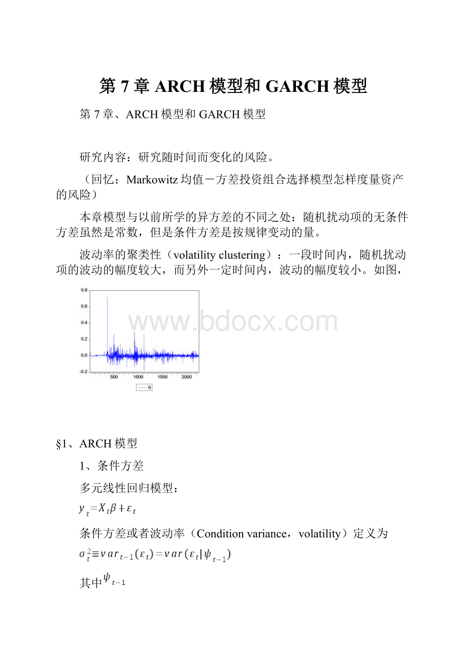
波动率的聚类性（volatilityclustering）：

一段时间内，随机扰动项的波动的幅度较大，而另外一定时间内，波动的幅度较小。

如图，

§1、ARCH模型

1、条件方差

多元线性回归模型：

条件方差或者波动率（Conditionvariance，volatility）定义为

其中

是信息集。

2、ARCH模型的定义

Engle（1982）提出ARCH模型（autoregressiveconditionalheteroskedasticity，自回归条件异方差）。

ARCH（q）模型：

（1）

的无条件方差是常数，但是其条件分布为

（2）

其中

是信息集。

方程

（1）是均值方程（meanequation）

✓

：

条件方差，含义是基于过去信息的一期预测方差

方程

（2）是条件方差方程（conditionalvarianceequation），由二项组成

✓常数

✓ARCH项

：

滞后的残差平方

习题：

方程

（2）给出了

的条件方差，请计算

的无条件方差。

证明：

利用方差分解公式：

Var（X）=VarY[E（X|Y）]+EY[Var（X|Y）]

由于

，所以条件均值为0，条件方差为

。

那么，

推出

，说明

3、ARCH模型的平稳性条件

在ARCH

（1）模型中，观察参数

的含义：

当

时，

当

时，退化为传统情形，

ARCH模型的平稳性条件：

（这样才得到有限的方差）

4、ARCH效应检验

ARCHLMTest：

拉格朗日乘数检验

建立辅助回归方程

此处

是回归残差。

原假设：

H0：

序列不存在ARCH效应

即

H0：

可以证明：

若H0为真，则

此处，m为辅助回归方程的样本个数。

R2为辅助回归方程的确定系数。

Eviews操作：

①先实施多元线性回归

②view/residual/Tests/ARCHLMTest

§2、GARCH模型的实证分析

从收盘价，得到收益率数据序列。

seriesr=log（p）-log（p（-1））

点击序列p，然后view/linegraph

1、检验是否有ARCH现象。

首先回归。

取2000到2254的样本。

输入lsrc，得到

DependentVariable:

R

Method:

LeastSquares

Date:

10/21/04Time:

21:

26

Sample:

20002254

Includedobservations:

255

Variable

Coefficient

Std.Error

t-Statistic

Prob.

C

0.000432

0.001087

0.397130

0.6916

R-squared

0.000000

Meandependentvar

0.000432

AdjustedR-squared

0.000000

S.D.dependentvar

0.017364

S.E.ofregression

0.017364

Akaikeinfocriterion

-5.264978

Sumsquaredresid

0.076579

Schwarzcriterion

-5.251091

Loglikelihood

672.2847

Durbin-Watsonstat

2.049819

问题：

这样进行回归的含义是什么？

其次，view/residualtests/ARCHLMtest，得到

ARCHTest:

F-statistic

5.220573

Probability

0.000001

Obs*R-squared

44.68954

Probability

0.000002

TestEquation:

DependentVariable:

RESID^2

Method:

LeastSquares

Date:

10/21/04Time:

21:

27

Sample（adjusted）:

20102254

Includedobservations:

245afteradjustingendpoints

Variable

Coefficient

Std.Error

t-Statistic

Prob.

C

0.000110

5.34E-05

2.060138

0.0405

RESID^2（-1）

0.141549

0.065237

2.169776

0.0310

RESID^2（-2）

0.055013

0.065823

0.835766

0.4041

RESID^2（-3）

0.337788

0.065568

5.151697

0.0000

RESID^2（-4）

0.026143

0.069180

0.377893

0.7059

RESID^2（-5）

-0.041104

0.069052

-0.595260

0.5522

RESID^2（-6）

-0.069388

0.069053

-1.004854

0.3160

RESID^2（-7）

0.005617

0.069178

0.081193

0.9354

RESID^2（-8）

0.102238

0.065545

1.559806

0.1202

RESID^2（-9）

0.011224

0.065785

0.170619

0.8647

RESID^2（-10）

0.064415

0.065157

0.988613

0.3239

R-squared

0.182406

Meandependentvar

0.000305

AdjustedR-squared

0.147466

S.D.dependentvar

0.000679

S.E.ofregression

0.000627

Akaikeinfocriterion

-11.86836

Sumsquaredresid

9.19E-05

Schwarzcriterion

-11.71116

Loglikelihood

1464.875

F-statistic

5.220573

Durbin-Watsonstat

2.004802

Prob（F-statistic）

0.000001

得到什么结论？

2、模型定阶：

如何确定q

实施ARCHLMtest时，取较大的q，观察滞后残差平方的t统计量的p－value即可。

此处选取q＝3。

因此，可以对残差建立ARCH（3）模型。

3、ARCH模型的参数估计

参数估计采用最大似然估计。

具体方法在GARCH一节中讲解。

如何实施ARCH过程：

由于存在ARCH效应，所以点击estimate，在method中选取ARCH

得到如下结果

DependentVariable:

R

Method:

ML-ARCH

Date:

10/21/04Time:

21:

48

Sample:

20002254

Includedobservations:

255

Convergenceachievedafter13iterations

Coefficient

Std.Error

z-Statistic

Prob.

C

-0.000640

0.000750

-0.852888

0.3937

VarianceEquation

C

9.24E-05

1.66E-05

5.569337

0.0000

ARCH

（1）

0.244793

0.082640

2.962142

0.0031

ARCH

（2）

0.081425

0.077428

1.051624

0.2930

ARCH（3）

0.457883

0.109698

4.174043

0.0000

R-squared

-0.003823

Meandependentvar

0.000432

AdjustedR-squared

-0.019884

S.D.dependentvar

0.017364

S.E.ofregression

0.017535

Akaikeinfocriterion

-5.495982

Sumsquaredresid

0.076872

Schwarzcriterion

-5.426545

Loglikelihood

705.7377

Durbin-Watsonstat

2.042013

为了比较，观察将q放大对系数估计的影响

DependentVariable:

R

Method:

ML-ARCH

Date:

10/21/04Time:

21:

54

Sample:

20002254

Includedobservations:

255

Convergenceachievedafter16iterations

Coefficient

Std.Error

z-Statistic

Prob.

C

-0.000601

0.000751

-0.799909

0.4238

VarianceEquation

C

9.38E-05

1.60E-05

5.880741

0.0000

ARCH

（1）

0.262009

0.090256

2.902959

0.0037

ARCH

（2）

0.041930

0.070518

0.594596

0.5521

ARCH（3）

0.452187

0.108488

4.168076

0.0000

ARCH（4）

-0.021920

0.050982

-0.429956

0.6672

ARCH（5）

0.037620

0.044394

0.847408

0.3968

R-squared

-0.003550

Meandependentvar

0.000432

AdjustedR-squared

-0.027830

S.D.dependentvar

0.017364

S.E.ofregression

0.017603

Akaikeinfocriterion

-5.483292

Sumsquaredresid

0.076851

Schwarzcriterion

-5.386081

Loglikelihood

706.1198

Durbin-Watsonstat

2.042568

观察：

说明q选取为3确实比较恰当。

4、ARCH模型是对的吗？

如果ARCH模型选取正确，即回归残差的条件方差是按规律变化的，那么标准化残差就会服从标准正态分布，即不会有ARCH效应了。

为什么？

请思考。

对q为3的ARCH模型做LMtest，发现没有了ARCH效应。

注意，虽然是同一个检验名称，但是ARCH过程后是对标准化残差进行检验。

注意观察被解释变量或者依赖变量是什么？

ARCHTest:

F-statistic

0.238360

Probability

0.992099

Obs*R-squared

2.470480

Probability

0.991299

TestEquation:

DependentVariable:

STD_RESID^2

Method:

LeastSquares

Date:

10/21/04Time:

21:

56

Sample（adjusted）:

20102254

Includedobservations:

245afteradjustingendpoints

Variable

Coefficient

Std.Error

t-Statistic

Prob.

C

1.102371

0.264990

4.160043

0.0000

STD_RESID^2（-1）

-0.038545

0.065360

-0.589741

0.5559

STD_RESID^2（-2）

-0.003804

0.065308

-0.058252

0.9536

STD_RESID^2（-3）

-0.057313

0.065303

-0.877649

0.3810

STD_RESID^2（-4）

-0.010325

0.065277

-0.158169

0.8745

STD_RESID^2（-5）

0.003537

0.065280

0.054185

0.9568

STD_RESID^2（-6）

-0.007420

0.065274

-0.113670

0.9096

STD_RESID^2（-7）

0.063317

0.065264

0.970165

0.3330

STD_RESID^2（-8）

-0.012167

0.065293

-0.186340

0.8523

STD_RESID^2（-9）

-0.010653

0.065278

-0.163194

0.8705

STD_RESID^2（-10）

-0.020211

0.065228

-0.309845

0.7570

R-squared

0.010084

Meandependentvar

1.007544

AdjustedR-squared

-0.032221

S.D.dependentvar

2.112747

S.E.ofregression

2.146514

Akaikeinfocriterion

4.409426

Sumsquaredresid

1078.160

Schwarzcriterion

4.566625

Loglikelihood

-529.1546

F-statistic

0.238360

Durbin-Watsonstat

2.000071

Prob（F-statistic）

0.992099

方程整体是不显著的。

还可以观察标准化残差

ARCH建模以后，procs/makeresidualseries/可以产生残差

和标准化残差

，以分别下是残差和标准化残差。

可以看出没有了集群现象。

还可以观察波动率（条件方差）的图形。

对比r和残差的图形，发现条件方差的起伏与波动率的大小一致。

ARCH建模以后，procs/makegarchvarianceseries/得到

结论：

ARCH模型确实很好描述了股票市场收益率的波动性。

可以观察系数之和小于1，满足平稳性条件。

§3、GARCH模型

当q较大时，采用Bollerslov（1986）提出的GARCH模型（GeneralizedARCH）

1、模型定义

条件方差方程

✓均值

✓

✓

：

过去的条件方差（也即预测方差，forecastvariance）

注意：

均值方程中若没有解释变量（即只有常数，如RC），则R2没有直观定义了，因此可为负）

2、GARCH（p,q）模型的稳定性条件

计算扰动项的无条件方差：

GARCH是协方差稳定的，因此是经典回归。

3、GARCH模型的参数估计

采用极大似然估计GARCH模型的参数。

下面以GARCH（1,1）为例。

由GARCH（1,1）模型

可以得到yt的分布为

由正态分布的定义公式，得到yt的pdf为

第t个观察样本的对数似然函数值为

其中

注意yi和yj之间不相关，因而是独立的。

似然函数为

取对数就得到了所有样本的对数似然函数。

其中条件方差项以非线性方式进入似然函数，所以不得不使用迭代算法求解。

4、模型的选择

两条原则：

1）若ARCH（q）中q太大，比如q大于7时，则选择GARCH（p,q）

2）使用AIC和SC准则，选择最优的GARCH模型

3）对于金融时间序列，一般选择GARCH（1,1）就够了。

回顾AIC和SC定义：

1）AIC准则（Akaikeinformationcriterion）

AIC越小越好，结合如下两者：

K（自变量个数）减少，模型简洁

LnL增加，模型精确

2）SC准则（Schwazcriterion）

习题1：

通货膨胀率有ARCH效应吗？

GreeneP572

点击数据文件usinf_greene_p572。

进行回归

lsinflationcinflation（-1）

DependentVariable:

INFLATION

Method:

LeastSquares

Date:

11/19/04Time:

10:

37

Sample（adjusted）:

19411985

Includedobservations:

45afteradjustingendpoints

Variable

Coefficient

Std.Error

t-Statistic

Prob.

C

2.432859

0.816345

2.980184

0.0047

INFLATION（-1）

0.493213

0.131157

3.760466

0.0005

R-squared

0.247477

Meandependentvar

4.740000

AdjustedR-squared

0.229976

S.D.dependentvar

4.116784

S.E.ofregression

3.612519

Akaikeinfocriterion

5.450114

Sumsquaredresid

561.1625

Schwarzcriterion

5.530410

Loglikelihood

-120.6276

F-statistic

14.14110

Durbin-Watsonstat

1.612442

Prob（F-statistic）

0.000507

检验ARCH效应

ARCHTest:

F-statistic

0.215950

Probability

0.953308

Obs*R-squared

1.231192

Probability

0.941850

TestEquation:

DependentVariable:

RESID^2

Method:

LeastSquares

Date:

11/19/04Time:

10:

46

Sample（adjusted）:

19461985

Includedobservations:

40afteradjustingendpoints

Variable

Coefficient

Std.Error

t-Statistic

Prob.

C

9.270522

7.425567

1.248460

0.2204

RESID^2（-1）

-0.031162

0.170116

-0.183184

0.8557

RESID^2（-2）

-0.006886

0.170151

-0.040469

0.9680

RESID^2（-3）

0.116261

0.169505

0.685888

0.4974

RESID^2（-4）

0.018545

0.170620

0.108694

0.9141

RESID^2（-5）

0.127906

0.168643

0.758439

0.4534

R-squared

0.030780

Meandependentvar

12.28323

AdjustedR-squared

-0.111753

S.D.dependentvar

34.15088

S.E.ofregression

36.00858

Akaikeinfocriterion

10.14287

Sumsquaredresid

44085.00

Schwarzcriterion

10.39620

Loglikelihood

-196.8574

F-statistic

0.215950

Durbin-Watsonstat

1.034796

Prob（F-statistic）

0.953308

习题2：

通货膨胀率有ARCH效应吗？

Lin的数据集

点击usinf文件

seriesdp=100*D（log（p））

lsdpcdp（-1）dp（-2）dp（-3）

DependentVariable:

DP

Method:

LeastSquares

Date:

11/19/04Time:

10:

10

Sample（adjusted）:

1951:

11983:

4

Includedobservations:

132afteradjustingendpoints

Variable

Coefficient

Std.Error

t-Statistic

Prob.

C

0.109907

0.063405

1.733410

0.0854

DP（-1）

0.393583

0.084432

4.661536

0.0000

DP（-2）

0.203093

0.089452

2.270405

0.0249

DP（-3）

0.302073

0.084185

3.588214

0.0005

R-squared

0.696825

Meandependentvar

1.021373

AdjustedR-squared

0.689719

S.D.dependentvar

0.711412

S.E.ofregression

0.396277

Akaikeinfocriterion

1.016428

Sumsquaredresid

20.10054

Schwarzcriterion

1.103785

Loglikelihood

-63.08423

F-statistic

98.06599

D