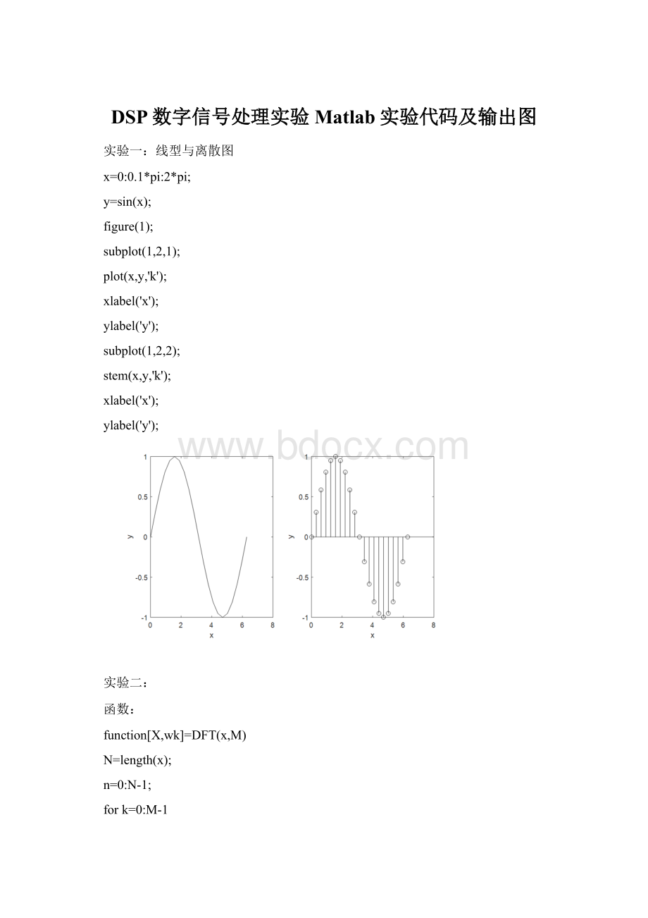
DSP数字信号处理实验Matlab实验代码及输出图Word下载.docx
《DSP数字信号处理实验Matlab实验代码及输出图Word下载.docx》由会员分享,可在线阅读,更多相关《DSP数字信号处理实验Matlab实验代码及输出图Word下载.docx(21页珍藏版)》请在冰豆网上搜索。
n=0:
N-1;
fork=0:
M-1
wk(k+1)=2*pi/M*k;
X(k+1)=sum(x.*exp(-j*wk(k+1)*n));
end
clc;
clearall;
A=444.128;
a=50*sqrt
(2)*pi;
w0=50*sqrt
(2)*pi;
fs=input('
输入采样频率fs='
T=1/fs;
N=50;
xa=A*exp(-a*n*T).*sin(w0*n*T);
stem(n,xa,'
.'
grid;
M=100;
[Xa,wk]=DFT(xa,M);
f=wk*fs/(2*pi);
plot(f,abs(Xa));
1000hz
500hz
200hz
DFT程序:
Clc
clearall
xbn=[1,0,0,0];
hbn=[1,2.5,2.5,1]
N=4;
Xb=fft(xbn,N);
Xh=fft(hbn,N);
ybn=conv(xbn,hbn);
subplot(3,2,1);
stem(n,xbn,'
title('
xbnwave'
subplot(3,2,2);
stem(n,abs(Xb),'
Xbwave'
subplot(3,2,3);
stem(n,hbn,'
hbnwave'
subplot(3,2,4);
stem(n,abs(Xh),'
Xhwave'
n1=0:
6;
Xy=fft(ybn,8);
subplot(3,2,5);
stem(n1,ybn,'
ybnwave'
)
n2=0:
7;
subplot(3,2,6);
stem(n2,abs(Xy),'
Xywave
结果:
hbn=
1.00002.50002.50001.0000
实验三:
第一个方程:
a1=[1,0.75,0.125];
b1=[1,-1];
20;
x1=[1zeros(1,20)];
subplot(2,3,1);
y1filter=filter(b1,a1,x1);
stem(n,y1filter);
ylfilter'
x1=[1zeros(1,10)];
[h]=impz(b1,a1,10);
subplot(2,3,2);
y1conv=conv(h,x1);
19;
stem(n,y1conv,'
filled'
subplot(2,3,3);
impz(b1,a1,21);
x2=ones(1,21);
subplot(2,3,4);
y1filter=filter(b1,a1,x2);
y1filter_step'
[h]=impz(b1,a1,20);
y1=conv(h,x2);
y1conv=y1(1:
21);
subplot(2,3,5);
stem(n1,y1conv,'
y1conv'
n'
y1[n]'
subplot(2,3,6);
b1=1;
impz(b1,a1);
第二个方程:
a1=[1];
b1=[0.25,0.25,0.25,0.25];
x1=[1zeros(1,20)];
y1filter'
[h]=impz(b1,a1,10);
impz(b1,a1,21);
a1=1;
b1=[0,0.25,0.5,0.75,ones(1,17)];
第一个方程结果
第二个方程结果:
实验四:
程序:
num=[0.05280.07970.12950.12950.7970.0528];
den=[1-1.81072.4947-1.88010.9537-0.2336];
[z,p,k]=tf2zp(num,den);
m=abs(p);
disp('
零点'
disp(z);
极点'
disp(p);
增益系数'
disp(k);
sos=zp2sos(z,p,k);
figure
(1)
zplane(num,den)
k=256;
w=0:
pi/k:
pi;
h=freqz(num,den,w);
plot(w/pi,real(h));
grid
实部'
\omega/\pi'
幅度'
plot(w/pi,imag(h));
虚部'
Amplitude'
plot(w/pi,abs(h));
幅度谱'
幅值'
plot(w/pi,angle(h));
相位谱'
弧度'
figure
(2)
freqz(num,den,128);
零点
-1.5870+1.4470i
-1.5870-1.4470i
0.8657+1.5779i
0.8657-1.5779i
-0.0669+0.0000i
极点
0.2788+0.8973i
0.2788-0.8973i
0.3811+0.6274i
0.3811-0.6274i
0.4910+0.0000i
增益系数
0.0528
实验五:
wp=input('
通带内频率wp='
ap=input('
容许幅度误差ap='
ws=input('
频率ws='
as=input('
阻带衰减as='
fs=1;
[N,Wn]=buttord(wp,ws,ap,as,'
s'
[Z,P,K]=buttap(N);
[Bap,Aap]=zp2tf(Z,P,K);
[b,a]=lp2lp(Bap,Aap,Wn);
[bz,az]=bilinear(b,a,fs);
[H,W]=freqz(bz,az,64);
subplot(2,1,1);
stem(W/pi,abs(H));
频率'
subplot(2,1,2);
stem(W/pi,20*log10(abs(H)));
幅度(dB)'
bz
az
结果:
通带内频率wp=0.1*pi
容许幅度误差ap=0.5
频率ws=0.5*pi
阻带衰减as=20
bz=
0.02380.07140.07140.0238
az=
1.0000-1.62171.0505-0.2384
实验六:
Blackman方式:
b=fir1(21,0.5,blackman(22));
y=freqz(b,1);
subplot(2,2,1);
plot(abs(y));
幅度响应'
subplot(2,2,2);
plot(angle(y));
相位响应'
subplot(2,2,3);
cj=impz(b,1,20);
stem(cj);
冲激响应'
Hamming方式:
b=fir1(21,0.5,hamming(22));
Hanning方式:
b=fir1(21,0.5,hanning(22));
cj=i
 升级会员
升级会员 