matlab习题.docx
《matlab习题.docx》由会员分享,可在线阅读,更多相关《matlab习题.docx(33页珍藏版)》请在冰豆网上搜索。
matlab习题
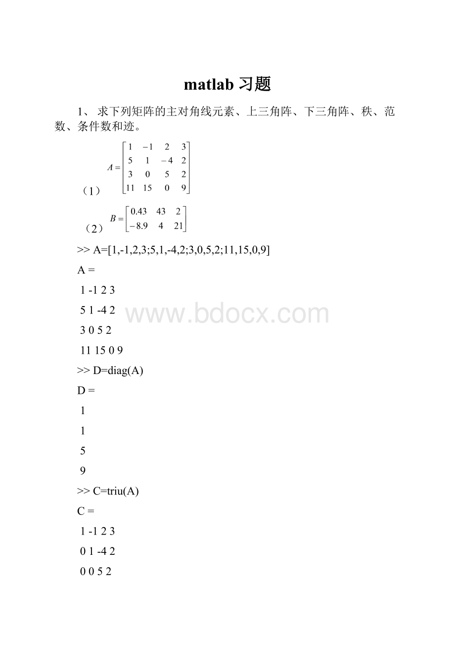
1、求下列矩阵的主对角线元素、上三角阵、下三角阵、秩、范数、条件数和迹。
(1)
(2)
>>A=[1,-1,2,3;5,1,-4,2;3,0,5,2;11,15,0,9]
A=
1-123
51-42
3052
111509
>>D=diag(A)
D=
1
1
5
9
>>C=triu(A)
C=
1-123
01-42
0052
0009
>>B=tril(A)
B=
1000
5100
3050
111509
>>E=rank(A)
E=
4
>>F=trace(A)
F=
16
>>a1=norm(A,1)
a1=
20
>>a2=norm(A,2)
a2=
21.3005
>>a3=norm(A,inf)
a3=
35
>>c1=cond(A)
c1=
11.1739
>>c1=cond(A,1)
c1=
14.4531
>>c2=cond(A,2)
c2=
11.1739
>>c3=cond(A,inf)
c3=
22.0938
>>
>>D=diag(B)
D=
0.4300
4.0000
>>C=triu(B)
C=
0.430043.00002.0000
04.000021.0000
>>A=tril(B)
A=
0.430000
-8.90004.00000
>>E=rank(B)
E=
2
>>F=trace(B)
F=
4.4300
>>a1=norm(B,1)
a1=
47
>>a2=norm(B,2)
a2=
43.4271
>>a3=norm(B,inf)
a3=
45.4300
>>c1=cond(B,1)
?
?
?
Errorusing==>cond
Aisrectangular.Usethe2norm.
>>c2=cond(B,2)
c2=
1.9354
>>c3=cond(B,inf)
?
?
?
Errorusing==>cond
Aisrectangular.Usethe2norm.
>>
2、求矩阵A的特征值和相应的特征向量。
>>A=[1,1,0.5;1,1,0.25;0.5,0.25,2]
A=
1.00001.00000.5000
1.00001.00000.2500
0.50000.25002.0000
>>[V,D]=eig(A)
V=
0.72120.44430.5315
-0.68630.56210.4615
-0.0937-0.69760.7103
D=
-0.016600
01.48010
002.5365
>>
3、下面是一个线性方程组:
(1)求方程的解。
(2)将方程右边向量元素
改为0.53,再求解,并比较
的变化和解的相对变化。
(3)计算系数矩阵A的条件数并分析结论。
>>A=[1/2,1/3,1/4;1/3,1/4,1/5;1/4,1/5,1/6]
A=
0.50000.33330.2500
0.33330.25000.2000
0.25000.20000.1667
>>b=[0.95,0.67,0.52]'
b=
0.9500
0.6700
0.5200
>>x=inv(A)*b
x=
1.2000
0.6000
0.6000
>>b=[0.95,0.67,0.53]'
b=
0.9500
0.6700
0.5300
>>x=inv(A)*b
x=
3.0000
-6.6000
6.6000
>>c1=cond(A,1)
c1=
2.0150e+003
>>c2=cond(A,2)
c2=
1.3533e+003
>>c3=cond(A,inf)
c3=
2.0150e+003
>>
4、利用Matlab提供的randn函数生成符合正态分布的10×5随机矩阵A,进行如下操作:
(1)A各列元素的均值和标准方差
(2)A的最大元素和最小元素
(3)求A每行元素的和以及全部元素之和
(4)分别对A的每列元素按升序、每行按降序排列
>>X=randn(10,5)
X=
-0.4326-0.18670.2944-0.3999-1.6041
-1.66560.7258-1.33620.69000.2573
0.1253-0.58830.71430.8156-1.0565
0.28772.18321.62360.71191.4151
-1.1465-0.1364-0.69181.2902-0.8051
1.19090.11390.85800.66860.5287
1.18921.06681.25401.19080.2193
-0.03760.0593-1.5937-1.2025-0.9219
0.3273-0.0956-1.4410-0.0198-2.1707
0.1746-0.83230.5711-0.1567-0.0592
>>M=mean(X)
M=
0.00130.23100.02530.3588-0.4197
>>D=std(X)
D=
0.90340.88291.18980.78321.0821
>>m=max(X)
m=
1.19092.18321.62361.29021.4151
>>n=min(X)
n=
-1.6656-0.8323-1.5937-1.2025-2.1707
>>p=sum(X,2)
p=
-2.3288
-1.3287
0.0105
6.2215
-1.4895
3.3602
4.9201
-3.6964
-3.3998
-0.3025
>>sum(p)
ans=
1.9666
>>
5、按要求对指定函数进行插值
(1)按下表用三次样条方法插值计算0~900范围内整数点的正弦值和0~750范围内整数点的正切值。
表1特殊角的正弦与正切值表
(度)
0
15
30
45
60
75
90
0
0.2588
0.5000
0.7071
0.8660
0.9659
1.0000
0
0.2679
0.5774
1.0000
1.7320
3.7320
>>x=0:
15*pi/180:
pi/2;
>>sin(x)
ans=
00.25880.50000.70710.86600.96591.0000
>>tan(x)
ans=
1.0e+016*
00.00000.00000.00000.00000.00001.6331
>>formatlong
>>interp1(x,sin(x),'spline')
ans=
Columns1through4
-0.26179938779915-0.19404072024055-0.130********957-0.07667926537588
Columns5through7
-0.03507446726987-0.008920597817280
>>interp1(x,tan(x),'spline')
ans=
1.0e+032*
Columns1through4
-0.00000000000000-0.00000000000000-0.00000000000000-0.00000000000000
Columns5through7
0.000000000000000.000000000000007.25368882144637
>>
(2)用三次多项式方法插值计算1~100之间整数的平方根
表21~100内特殊值的平方根
1
4
9
16
25
36
49
64
81
100
1
2
3
4
5
6
7
8
9
10
>>N=[149162536496481100]
N=
149162536496481100
>>n=sqrt(N)
n=
12345678910
>>formatlong
>>interp1(N,n,'cubic')
ans=
149162536496481100
>>
6、将10个学生5门功课的成绩存入矩阵P中,进行如下处理:
(1)分别求每门功课的最高分、最低分及相应的学号。
(2)分别求每门功课的平均值和标准方差。
(3)5门课总分的最高分、最低分及相应的学号。
(4)将5门课总分按从大到小的顺序存入abc中,相应的学生序号存入mmw。
提示:
为了避免输入学生成绩的麻烦,可用取值范围在[45,95]之间的随机矩阵来表示学生成绩。
>>x=45+(95-45)*rand(5,10)
x=
Columns1through9
92.506583.104875.771665.285347.894655.138345.763765.932586.9059
56.556967.823484.596991.773562.643454.936182.339387.311145.9820
75.342145.925291.090690.845285.658375.189667.254871.257679.0639
69.299186.070481.910465.513545.493158.609491.590755.132463.9741
89.564967.235253.813389.682551.944554.940768.299778.606986.5898
Column10
70.1406
80.4736
66.4446
60.2309
54.4827
>>m1=max(x,[],2)
m1=
92.5065
91.7735
91.0906
91.5907
89.6825
>>[m1,l1]=max(x,[],2)
m1=
92.5065
91.7735
91.0906
91.5907
89.6825
l1=
1
4
3
7
4
>>m2=min(x,[],2)
m2=
45.7637
45.9820
45.9252
45.4931
51.9445
>>[m2,l2]=min(x,[],2)
m2=
45.7637
45.9820
45.9252
45.4931
51.9445
l2=
7
9
2
5
5
>>x1=mean(x)
x1=
Columns1through9
76.653970.031877.436680.620058.726859.762871.049671.648172.5031
Column10
66.3545
>>x2=std(x)
x2=
Columns1through9
14.813015.984114.305113.914416.42498.764317.397812.240717.5002
Column10
9.9011
>>n1=sum(x,2)
n1=
688.4438
714.4360
748.0721
677.8238
695.1602
>>n2=sum(x,1)
n2=
Columns1through9
383.2696350.1589387.1828403.1000293.6339298.8141355.2482358.2404362.5156
Column10
331.7724
>>[n2,l3]=max(x,[],1)
n2=
Columns1through9
92.506586.070491.090691.773585.658375.189691.590787.311186.9059
Column10
80.4736
l3=
1432334212
>>
7、某气象站观测某日6:
00~8:
00之间每隔2h内温度(0C)如实验表1所示
实验表1室内外温度观测结果(0C)
时间h
6
8
10
12
14
16
18
室内温度t1
18.0
20.0
22.0
25.0
30.0
28.0
24.0
室外温度t2
15.0
19.0
24.0
28.0
34.0
32.0
30.0
试用三次样条插值分别求出该日室内外6:
30~17:
30之间每隔2h各个点的近似温度(0C)。
>>h=6:
2:
18;
>>t1=[18202225302824]
t1=
18202225302824
>>t2=[15192428343230]
t2=
15192428343230
>>formatlong
>>interp1(h,t1,'spline')
ans=
Columns1through4
40.0000000000007044.0000000000011348.0000000000017154.00000000000289
Columns5through7
64.0000000000058860.0000000000045152.00000000000244
>>interp1(h,t2,'spline')
ans=
Columns1through4
34.0000000000002842.0000000000009052.0000000000024460.00000000000451
Columns5through7
72.0000000000094168.0000000000075064.00000000000588
>>
8、已知一组实验数据如下表所示:
一组实验数据
i
1
2
3
4
5
xi
165
123
150
123
141
yi
187
126
172
125
148
求它的线性拟合曲线。
>>i=1:
5
i=
12345
>>x=[165126172125148]
x=
165126172125148
>>y=[187126172125148]
y=
187126172125148
>>b=ployfit(x,y,2)
?
?
?
Undefinedcommand/function'ployfit'.
>>polyfit(x,y,2)
ans=
-0.00623.0359-158.5931
>>m=polyfit(x,y,2)
m=
-0.00623.0359-158.5931
>>n=polyval(m,x)
n=
173.5034125.4802180.1261124.0008154.8894
>>plot(x,n,'m-')
>>
9、已知
在【1,101】区间10个整数采样点的函数值如实验表所示:
在10个整数采样点的函数值
1
11
21
31
41
51
61
71
81
91
101
0
1.0414
1.3222
1.4914
1.6128
1.7076
1.7853
1.8513
1.9085
1.9590
2.0043
试求
的5次拟合多项式
,并绘制出
和
在【1,101】区间的函数曲线。
>>x=1:
10:
101
x=
1112131415161718191101
>>y=log10(x)
y=
Columns1through9
01.04141.32221.49141.61281.70761.78531.85131.9085
Columns10through11
1.95902.0043
>>p=polyfit(x,y,5)
Warning:
Polynomialisbadlyconditioned.Removerepeateddatapoints
ortrycenteringandscalingasdescribedinHELPPOLYFIT.
>Inpolyfitat81
p=
0.0000-0.00000.0001-0.00580.1537-0.1326
>>plot(p)
>>
>>plot(y)
>>
10、已知多项式
,
,
,求:
(1)
。
(2)
的全部根。
(3)计算
各点上的
。
>>x1=[3,2];x2=[5,-1,2];
>>x3=[1,0,-0.5];
>>c=conv(x1,x2)
c=
15744
>>d=conv(c,x3)
d=
15.00007.0000-3.50000.5000-2.0000-2.0000
>>x=roots(d)
x=
0.7071
0.1000+0.6245i
0.1000-0.6245i
-0.7071
-0.6667
>>m=[0,0.2i,0.4i,0.6i,0.8i,i,1.2i,1.4i,1.6i,1.8i,2i]
m=
Columns1through5
00+0.2000i0+0.4000i0+0.6000i0+0.8000i
Columns6through10
0+1.0000i0+1.2000i0+1.4000i0+1.6000i0+1.8000i
Column11
0+2.0000i
>>y=polyval(d,m)
y=
1.0e+002*
Columns1through5
-0.0200-0.0201-0.0037i-0.0190-0.0042i-0.0127+0.0072i0.0055+0.0511i
Columns6through10
0.0450+0.1650i0.1180+0.4097i0.2391+0.8748i0.4260+1.6842i0.6986+3.0025i
Column11
1.0800+5.0400i
>>
11、求函数在指定点的数值导数:
(1)
>>symsx
>>y=(sin(x))^2+(cos(x))^2;
>>dy=diff(y);
>>x=[pi/6,pi/4,pi/3,pi/2];
>>eval(dy)
ans=
0
>>
(2)
>>symsx
>>y=sqrt(1+x^2);
>>dy=diff(y);
>>x=1
x=
1
>>eval(dy)
ans=
0.7071
>>x=2
x=
2
>>eval(dy)
ans=
0.8944
>>x=3
x=
3
>>eval(dy)
ans=
0.9487
>>
12,求数值积分:
(1)
>>a=-1;b=1;
>>n=100;h=(b-a)/n;
>>x=a;s=0;
>>f0=(1+x^2)/(1+x^4);
>>fori=1:
n
x=x+h;
f1=(1+x^2)/(1+x^4);
s=s+(f0+f1)*h/2;
f0=f1;
end
>>s
s=
2.2214
>>
(2)
>>a=0;b=pi;
>>n=1000;h=(b-a)/n;
>>x=a;s=0;
>>f0=(log2(1+x))/(1+(cos(x))^2);
>>fori=1:
n
x=x+h;
f1=(log2(1+x))/(1+(cos(x))^2);
s=s+(f0+f1)*h/2;
f0=f1;
end
>>s
s=
2.8461
>>
(3)
>>a=0;b=pi;
>>n=10000;h=(b-a)/n;
>>x=a;s=0;
>>f0=(x*sin(x))/(1+x^2);
>>fori=1:
n
x=x+h;
f1=(x*sin(x))/(1+x^2);
s=s+(f0+f1)*h/2;
f0=f1;
end
>>s
s=
0.8415
>>
已知
,取
,对
从
采样,用FFT做快速傅立叶变换,并绘制出相应的振幅和频率图。
>>N=64;
>>T=5;
>>t=linspace(0,T,N);
>>x=exp(-t);
>>dt=t
(2)-t
(1);
>>f=1/dt;
>>X=fft(x);
>>F=X(1:
N/2+1);
>>f=f*(0:
N/2);
>>plot(f,abs(F),'-*')
>>
1.写出完成下列操作的命令:
1)将矩阵A的第2~5行中的第1,3,5列元素赋给矩阵B
答
B=A(2:
5,1:
2:
5)
2)删除矩阵A的第7号元素
答
A(7)=[];
3)将矩阵A的每个元素值加30
答
A=A+30
4)求矩
 升级会员
升级会员 