计量经济作业.docx
《计量经济作业.docx》由会员分享,可在线阅读,更多相关《计量经济作业.docx(27页珍藏版)》请在冰豆网上搜索。
计量经济作业
计量经济学平时作业
第二章第十题
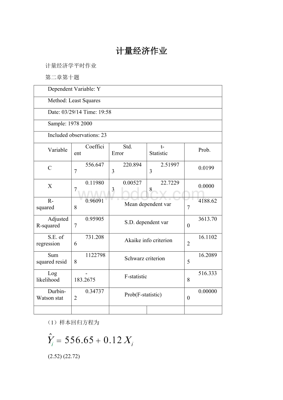
DependentVariable:
Y
Method:
LeastSquares
Date:
03/29/14Time:
19:
58
Sample:
19782000
Includedobservations:
23
Variable
Coefficient
Std.Error
t-Statistic
Prob.
C
556.6477
220.8943
2.519973
0.0199
X
0.119807
0.005273
22.72298
0.0000
R-squared
0.960918
Meandependentvar
4188.627
AdjustedR-squared
0.959057
S.D.dependentvar
3613.700
S.E.ofregression
731.2086
Akaikeinfocriterion
16.11022
Sumsquaredresid
11227988
Schwarzcriterion
16.20895
Loglikelihood
-183.2675
F-statistic
516.3338
Durbin-Watsonstat
0.347372
Prob(F-statistic)
0.000000
(1)样本回归方程为
(2.52)(22.72)
=0.96F=516.33
经济意义:
解释变量的系数为0.12,说明国内生产总值没增加1亿元,将有0.12亿元为财政收入,这是符合经济意义的。
散点图如下:
(2)
1).拟合优度检验:
=0.96
说明在总离差平方和中有96%的部分被回归直线解释,仅有4%未被解释,因此,样本回归直线对样本点的拟合优度较好。
2).显著性检验:
给出显著性水平
,自由度v=23-2=19,得临界值
=2.09
故t0=2.52>2.09t1=22.72>2.09,故回归系数均显著不为零,X对Y有显著影响。
(3)
点预测:
X=105709
故Y=13241.73
区间预测:
Y的区间预测为(11480.79,15000.67)
第三章第七题(课件)
DependentVariable:
Y
Method:
LeastSquares
Date:
04/1/14Time:
21:
11
Sample:
110
Includedobservations:
10
Variable
Coefficient
Std.Error
t-Statistic
Prob.
C
626.5093
40.13010
15.61195
0.0000
X1
-9.790570
3.197843
-3.061617
0.0183
X2
0.028618
0.005838
4.902030
0.0017
R-squared
0.902218
Meandependentvar
670.3300
AdjustedR-squared
0.874281
S.D.dependentvar
49.04504
S.E.ofregression
17.38985
Akaikeinfocriterion
8.792975
Sumsquaredresid
2116.847
Schwarzcriterion
8.883751
Loglikelihood
-40.96488
F-statistic
32.29408
Durbin-Watsonstat
1.650804
Prob(F-statistic)
0.000292
(1).估计参数
=626.5093,
=-9.790570,
=0.028618
=302.41,
=0.902218,
=0.874281
(2).F检验:
:
由表可知,F统计量为32.29,给定显著性水平0.05,则
=4.74,因为F统计量大于4.74,所以拒绝原假设,总体回归方程是显著的,即该社区家庭消费支出与商品单价和家庭月收入之间在总体上存在显著的线性关系。
T检验:
由表可知,
,给定显著性水平0.05,查表得
=2.37,
和
的绝对值都大于2.37,所以否定
即商品单价对该社区家庭消费有显著影响,家庭月收入对该社区家庭消费也有显著影响。
置信区间:
经计算得
两个端点分别为-17.374和-2.206,
的两个端点分别为0.015和0.043,所以
95%的置信区间是(-17.374,-2.206),
95%的置信区间是(0.015,0.043)。
第四章第三题
由题意得:
两边取对数,可得到
令=,=,,=,=,=,=,
即可将原函数模型转化成标准的二元线性回归模型
W
X1
X2
8.222204
8.032107
4.727388
7.274147
7.429183
4.204693
7.468724
7.916724
4.430817
7.280208
7.587726
3.295837
8.546616
8.685587
5.789960
7.736814
7.472370
4.787492
7.204276
6.844922
4.060443
6.487334
6.543826
3.433987
5.913989
5.895724
2.772589
7.371716
7.828831
4.189655
6.424399
6.881134
4.060443
6.426391
6.246126
3.332205
8.395972
8.239042
4.110874
8.656785
9.069701
5.537334
7.485138
7.936982
4.418841
7.125339
7.500220
3.496508
6.700362
7.020021
3.761200
7.549451
7.626648
4.110874
8.214154
8.718191
5.480639
8.462293
9.130025
5.402677
7.687186
7.960899
4.382027
7.839825
7.842133
4.564348
8.021896
8.473847
5.402677
7.692857
8.088037
5.093750
DependentVariable:
Y
Method:
LeastSquares
Date:
04/07/14Time:
10:
02
Sample:
131
Includedobservations:
31
Variable
Coefficient
Std.Error
t-Statistic
Prob.
C
1.153994
0.727611
1.586004
0.1240
X1
0.609236
0.176378
3.454149
0.0018
X2
0.360796
0.201591
1.789741
0.0843
R-squared
0.809925
Meandependentvar
7.493997
AdjustedR-squared
0.796348
S.D.dependentvar
0.942960
S.E.ofregression
0.425538
Akaikeinfocriterion
1.220839
Sumsquaredresid
5.070303
Schwarzcriterion
1.359612
Loglikelihood
-15.92300
F-statistic
59.65501
Durbin-Watsonstat
0.793209
Prob(F-statistic)
0.000000
所以所得回归方程为
。
第五章第六题
DependentVariable:
Y
Method:
LeastSquares
Date:
04/21/14Time:
16:
40
Sample:
120
Includedobservations:
20
Variable
Coefficient
Std.Error
t-Statistic
Prob.
C
272.3635
159.6773
1.705713
0.1053
X
0.755125
0.023316
32.38690
0.0000
R-squared
0.983129
Meandependentvar
5199.515
AdjustedR-squared
0.982192
S.D.dependentvar
1625.275
S.E.ofregression
216.8900
Akaikeinfocriterion
13.69130
Sumsquaredresid
846743.0
Schwarzcriterion
13.79087
Loglikelihood
-134.9130
F-statistic
1048.912
Durbin-Watsonstat
1.301684
Prob(F-statistic)
0.000000
1.
即为人均消费支出与可支配收入之间的线性模型。
2.
怀特检验
WhiteHeteroskedasticityTest:
F-statistic
14.63595
Probability
0.000201
Obs*R-squared
12.65213
Probability
0.001789
因为TR*2>
=3.841,所以该回归模型中存在异方差。
由图示法也可以得到相同的结果。
3.
E1与X^1/2
DependentVariable:
E1
Method:
LeastSquares
Date:
04/21/14Time:
17:
18
Sample:
120
Includedobservations:
20
Variable
Coefficient
Std.Error
t-Statistic
Prob.
X^(1/2)
2.315339
0.243625
9.503697
0.0000
R-squared
0.326056
Meandependentvar
177.2539
AdjustedR-squared
0.326056
S.D.dependentvar
107.2046
S.E.ofregression
88.00868
Akaikeinfocriterion
11.84145
Sumsquaredresid
147165.0
Schwarzcriterion
11.89124
Loglikelihood
-117.4145
Durbin-Watsonstat
1.382822
E1与X
DependentVariable:
E1
Method:
LeastSquares
Date:
04/21/14Time:
17:
21
Sample:
120
Includedobservations:
20
Variable
Coefficient
Std.Error
t-Statistic
Prob.
X
0.028126
0.002424
11.60484
0.0000
R-squared
0.520566
Meandependentvar
177.2539
AdjustedR-squared
0.520566
S.D.dependentvar
107.2046
S.E.ofregression
74.22977
Akaikeinfocriterion
11.50091
Sumsquaredresid
104691.1
Schwarzcriterion
11.55070
Loglikelihood
-114.0091
Durbin-Watsonstat
1.960065
E1和X^2
DependentVariable:
E1
Method:
LeastSquares
Date:
04/21/14Time:
17:
24
Sample:
120
Includedobservations:
20
Variable
Coefficient
Std.Error
t-Statistic
Prob.
X^2
3.30E-06
3.29E-07
10.03804
0.0000
R-squared
0.384817
Meandependentvar
177.2539
AdjustedR-squared
0.384817
S.D.dependentvar
107.2046
S.E.ofregression
84.08445
Akaikeinfocriterion
11.75023
Sumsquaredresid
134333.7
Schwarzcriterion
11.80001
Loglikelihood
-116.5023
Durbin-Watsonstat
1.688103
EI和X^3/2
DependentVariable:
E1
Method:
LeastSquares
Date:
04/21/14Time:
17:
25
Sample:
120
Includedobservations:
20
Variable
Coefficient
Std.Error
t-Statistic
Prob.
X^(3/2)
0.000316
2.68E-05
11.78825
0.0000
R-squared
0.533588
Meandependentvar
177.2539
AdjustedR-squared
0.533588
S.D.dependentvar
107.2046
S.E.ofregression
73.21471
Akaikeinfocriterion
11.47338
Sumsquaredresid
101847.5
Schwarzcriterion
11.52316
Loglikelihood
-113.7338
Durbin-Watsonstat
2.093814
W=1/e
WhiteHeteroskedasticityTest:
F-statistic
0.032603
Probability
0.967983
Obs*R-squared
0.076420
Probability
0.962511
TestEquation:
DependentVariable:
STD_RESID^2
Method:
LeastSquares
Date:
04/25/14Time:
10:
09
Sample:
120
Includedobservations:
20
Variable
Coefficient
Std.Error
t-Statistic
Prob.
C
6196.481
11798.68
0.525184
0.6062
X
-0.165323
3.304793
-0.050025
0.9607
X^2
4.80E-06
0.000211
0.022745
0.9821
R-squared
0.003821
Meandependentvar
5342.798
AdjustedR-squared
-0.113377
S.D.dependentvar
3140.196
S.E.ofregression
3313.430
Akaikeinfocriterion
19.18684
Sumsquaredresid
1.87E+08
Schwarzcriterion
19.33620
Loglikelihood
-188.8684
F-statistic
0.032603
成立消除了异方差,所以
=6196.48,
=-0.165
W=1/x
WhiteHeteroskedasticityTest:
F-statistic
1.111395
Probability
0.351865
Obs*R-squared
2.312660
Probability
0.314639
TestEquation:
DependentVariable:
STD_RESID^2
Method:
LeastSquares
Date:
04/25/14Time:
10:
12
Sample:
120
Includedobservations:
20
Variable
Coefficient
Std.Error
t-Statistic
Prob.
C
-67139.63
78728.82
-0.852796
0.4056
X
25.38176
22.05183
1.151004
0.2657
X^2
-0.001467
0.001408
-1.042164
0.3119
R-squared
0.115633
Meandependentvar
29670.20
AdjustedR-squared
0.011590
S.D.dependentvar
22238.71
S.E.ofregression
22109.46
Akaikeinfocriterion
22.98288
Sumsquaredresid
8.31E+09
Schwarzcriterion
23.13224
Loglikelihood
-226.8288
F-statistic
1.111395
Durbin-Watsonstat
1.713243
Prob(F-statistic)
0.351865
消除了异方差,所以参数为
=-67139.63,
=25.38.
第六章第五题
1.一元线性模型
DependentVariable:
Y
Method:
LeastSquares
Date:
05/04/14Time:
08:
09
Sample:
19602001
Includedobservations:
42
Variable
Coefficient
Std.Error
t-Statistic
Prob.
C
-3028.563
655.4268
-4.620749
0.0000
X
0.697492
0.019060
36.59467
0.0000
R-squared
0.970997
Meandependentvar
10765.23
AdjustedR-squared
0.970272
S.D.dependentvar
20154.12
S.E.ofregression
3474.938
Akaikeinfocriterion
19.19099
Sumsquaredresid
4.83E+08
Schwarzcriterion
19.27373
Loglikelihood
-401.0108
F-statistic
1339.170
Durbin-Watsonstat
0.178439
Prob(F-statistic)
0.000000
一元线性回归估计方程Y=-3028.563+0.697x
2.残差图
3.DW=0.178439
一阶自相关检验存在
Breusch-GodfreySerialCorrelationLMTest:
F-statistic
327.3780
Probability
0.000000
Obs*R-squared
37.52921
Probability
0.000000
TestEquation:
DependentVariable:
RESID
Method:
LeastSquares
Date:
05/05/14Time:
08:
14
Presamplemissingvaluelaggedresidualssettozero.
Variable
Coefficient
Std.Error
t-Statistic
Prob.
C
-312.6482
221.1676
-1.413626
0.1656
X
0.026360
0.007930
3.324113
0.0020
RESID(-1)
1.366995
0.155705
8.779407
0.0000
RESID(-2)
-0.319088
0.178289
-1.789723
0.0815
R-squared
0.901828
Meandependentvar
-3.29E-12
AdjustedR-squared
0.894077
S.D.dependentvar
3432.299
S.E.ofregression
1117.068
Akaikeinfocriterion
16.96520
Sumsquaredresid
47417961
Schwarzcriterion
17.13069
Loglikelihood
-352.2691
F-statistic
116.3582
Durbin-Watsonstat
1.756459
Prob(F-statistic)
0.000000
P=1-0.178439/2=0.91
4.广义差分法
DependentVariable:
Y1
Method:
L
 升级会员
升级会员 