机器视觉2.docx
《机器视觉2.docx》由会员分享,可在线阅读,更多相关《机器视觉2.docx(21页珍藏版)》请在冰豆网上搜索。
机器视觉2
机器视觉与图像处理
实验报告
学院名称:
电气工程学院
专业班级:
自动F1205
学生姓名:
王国顺
学号:
201223911018
实验一
实验内容:
Matlab软件的使用
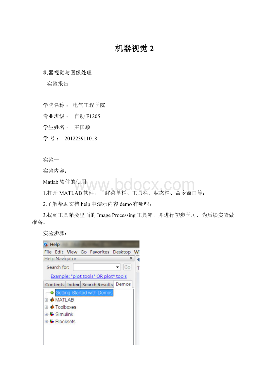
1.打开MATLAB软件,了解菜单栏、工具栏、状态栏、命令窗口等;
2.了解帮助文档help中演示内容demo有哪些;
3.找到工具箱类里面的ImageProcessing工具箱,并进行初步学习,为后续实验做准备。
实验步骤:
实验二
实验内容:
图像的增强技术
1.了解图像增强技术/方法的原理;
2.利用matlab软件,以某一用途为例,实现图像的增强;
3.通过程序的调试,初步了解图像处理命令的使用方法。
实验步骤:
pout=imread('pout.tif');
tire=imread('tire.tif');
[Xmap]=imread('shadow.tif');
shadow=ind2rgb(X,map);%converttotruecolor
width=210;
images={pout,tire,shadow};
fork=1:
3
dim=size(images{k});
images{k}=imresize(images{k},[width*dim
(1)/dim
(2)width],'bicubic');
End
pout=images{1};
tire=images{2};
shadow=images{3};
pout_imadjust=imadjust(pout);
pout_histeq=histeq(pout);
pout_adapthisteq=adapthisteq(pout);
imshow(pout);
title('Original');
figure,imshow(pout_imadjust);
title('Imadjust');
figure,imshow(pout_histeq);
title('Histeq');
figure,imshow(pout_adapthisteq);
title('Adapthisteq');
实验三
实验内容:
图像特征提取
1.了解图像特征提取的方法;
2.利用matlab软件,编程实现图像中长度、角度、半径、边界等特征的提取测量;
3.通过程序的调试,初步了解图像特征提取命令的使用方法。
实验步骤:
1.
loadpendulum;
immovie(frames);
nFrames=size(frames,4);
first_frame=frames(:
:
:
1);
first_region=imcrop(first_frame,rect);
frame_regions=repmat(uint8(0),[size(first_region)nFrames]);
forcount=1:
nFrames
frame_regions(:
:
:
count)=imcrop(frames(:
:
:
count),rect);
end
immovie(frame_regions);
seg_pend=false([size(first_region,1)size(first_region,2)nFrames]);
centroids=zeros(nFrames,2);
se_disk=strel('disk',3);
forcount=1:
nFrames
fr=frame_regions(:
:
:
count);
imshow(fr)
pause(0.2)
gfr=rgb2gray(fr);
gfr=imcomplement(gfr);
imshow(gfr)
pause(0.2)
bw=im2bw(gfr,.7);%thresholdisdeterminedexperimentally
bw=imopen(bw,se_disk);
bw=imclearborder(bw);
seg_pend(:
:
count)=bw;
imshow(bw)
pause(0.2)
end
forcount=1:
nFrames
lab=bwlabel(seg_pend(:
:
count));
property=regionprops(lab,'Centroid');
pend_centers(count,:
)=property.Centroid;
end
x=pend_centers(:
1);
y=pend_centers(:
2);
figure
plot(x,y,'m.'),axisij,axisequal,holdon;
xlabel('x');
ylabel('y');
title('pendulumcenters');
abc=[xyones(length(x),1)]\[-(x.^2+y.^2)];
a=abc
(1);b=abc
(2);c=abc(3);
xc=-a/2;
yc=-b/2;
circle_radius=sqrt((xc^2+yc^2)-c);
pendulum_length=round(circle_radius)
circle_theta=pi/3:
0.01:
pi*2/3;
x_fit=circle_radius*cos(circle_theta)+xc;
y_fit=circle_radius*sin(circle_theta)+yc;
plot(x_fit,y_fit,'b-');
plot(xc,yc,'bx','LineWidth',2);
plot([xcx
(1)],[ycy
(1)],'b-');
text(xc-110,yc+100,sprintf('pendulumlength=%dpixels',pendulum_length));
实验结果:
2.
RGB=imread('pillsetc.png');
imshow(RGB);
I=rgb2gray(RGB);
threshold=graythresh(I);
bw=im2bw(I,threshold);
imshow(bw)
%removeallobjectcontainingfewerthan30pixels
bw=bwareaopen(bw,30);
%fillagapinthepen'scap
se=strel('disk',2);
bw=imclose(bw,se);
%fillanyholes,sothatregionpropscanbeusedtoestimate
%theareaenclosedbyeachoftheboundaries
bw=imfill(bw,'holes');
imshow(bw)
[B,L]=bwboundaries(bw,'noholes');
%Displaythelabelmatrixanddraweachboundary
imshow(label2rgb(L,@jet,[.5.5.5]))
holdon
fork=1:
length(B)
boundary=B{k};
plot(boundary(:
2),boundary(:
1),'w','LineWidth',2)
end
stats=regionprops(L,'Area','Centroid');
threshold=0.94;
%loopovertheboundaries
fork=1:
length(B)
%obtain(X,Y)boundarycoordinatescorrespondingtolabel'k'
boundary=B{k};
%computeasimpleestimateoftheobject'sperimeter
delta_sq=diff(boundary).^2;
perimeter=sum(sqrt(sum(delta_sq,2)));
%obtaintheareacalculationcorrespondingtolabel'k'
area=stats(k).Area;
%computetheroundnessmetric
metric=4*pi*area/perimeter^2;
%displaytheresults
metric_string=sprintf('%2.2f',metric);
%markobjectsabovethethresholdwithablackcircle
ifmetric>threshold
centroid=stats(k).Centroid;
plot(centroid
(1),centroid
(2),'ko');
end
text(boundary(1,2)-35,boundary(1,1)+13,metric_string,'Color','y',...
'FontSize',14,'FontWeight','bold');
end
title(['Metricscloserto1indicatethat',...
'theobjectisapproximatelyround']);
实验结果:
3.
RGB=imread('gantrycrane.png');
imshow(RGB);
text(size(RGB,2),size(RGB,1)+15,'ImagecourtesyofJeffMather',...
'FontSize',7,'HorizontalAlignment','right');
line([300328],[85103],'color',[110]);
line([268255],[85140],'color',[110]);
text(150,72,'Measuretheanglebetweenthesebeams','Color','y',...
'FontWeight','bold');
%youcanobtainthecoordinatesoftherectangularregionusing
%pixelinformationdisplayedbyimtool
start_row=34;
start_col=208;
cropRGB=RGB(start_row:
163,start_col:
400,:
);
imshow(cropRGB)
%Store(X,Y)offsetsforlateruse;subtract1sothateachoffsetwill
%correspondtothelastpixelbeforetheregionofinterest
offsetX=start_col-1;
offsetY=start_row-1;
I=rgb2gray(cropRGB);
threshold=graythresh(I);
BW=im2bw(I,threshold);
BW=~BW;%complementtheimage(objectsofinterestmustbewhite)
imshow(BW)
dim=size(BW);
%horizontalbeam
col1=4;
row1=min(find(BW(:
col1)));
%angledbeam
row2=12;
col2=min(find(BW(row2,:
)));
boundary1=bwtraceboundary(BW,[row1,col1],'N',8,70);
%setthesearchdirectiontocounterclockwise,inordertotracedownward.
boundary2=bwtraceboundary(BW,[row2,col2],'E',8,90,'counter');
imshow(RGB);holdon;
%applyoffsetsinordertodrawintheoriginalimage
plot(offsetX+boundary1(:
2),offsetY+boundary1(:
1),'g','LineWidth',2);
plot(offsetX+boundary2(:
2),offsetY+boundary2(:
1),'g','LineWidth',2);
实验结果:
4.
RGB=imread('tape.png');
imshow(RGB);
text(15,15,'Estimateradiusoftherolloftape',...
'FontWeight','bold','Color','y');
I=rgb2gray(RGB);
threshold=graythresh(I);
BW=im2bw(I,threshold);
imshow(BW)
dim=size(BW);
col=round(dim
(2)/2)-90;
row=find(BW(:
col),1);
connectivity=8;
num_points=180;
contour=bwtraceboundary(BW,[row,col],'N',connectivity,num_points);
imshow(RGB);
holdon;
plot(contour(:
2),contour(:
1),'g','LineWidth',2)
x=contour(:
2);
y=contour(:
1);
%solveforparametersa,b,andcintheleast-squaressenseby
%usingthebackslashoperator
abc=[xyones(length(x),1)]\-(x.^2+y.^2);
a=abc
(1);b=abc
(2);c=abc(3);
%calculatethelocationofthecenterandtheradius
xc=-a/2;
yc=-b/2;
radius=sqrt((xc^2+yc^2)-c)
%displaythecalculatedcenter
plot(xc,yc,'yx','LineWidth',2);
%plottheentirecircle
theta=0:
0.01:
2*pi;
%useparametricrepresentationofthecircletoobtaincoordinates
%ofpointsonthecircle
Xfit=radius*cos(theta)+xc;
Yfit=radius*sin(theta)+yc;
plot(Xfit,Yfit);
message=sprintf('Theestimatedradiusis%2.3fpixels',radius);
text(15,15,message,'Color','y','FontWeight','bold');
实验结果:
实验四
实验内容:
图像变换
1.了解图像变换的原理;
2.利用matlab软件,编程实现投影数据的图像重构;
3.通过程序的调试,初步了解图像投影变换的应用。
实验步骤:
P=phantom(256);
imshow(P)
theta1=0:
10:
170;
[R1,xp]=radon(P,theta1);
num_angles_R1=size(R1,2)
theta3=0:
2:
178;
[R3,xp]=radon(P,theta3);
num_angles_R3=size(R3,2)
N_R1=size(R1,1)
N_R2=size(R2,1)
N_R3=size(R3,1)
P_128=phantom(128);
[R_128,xp_128]=radon(P_128,theta1);
N_128=size(R_128,1)
figure,imagesc(theta3,xp,R3)
colormap(hot)
colorbar
xlabel('ParallelRotationAngle-\theta(degrees)');
ylabel('ParallelSensorPosition-x\prime(pixels)');
%Constraintheoutputsizeofeachreconstructiontobethesameasthe
%sizeoftheoriginalimage,|P|.
output_size=max(size(P));
dtheta1=theta1
(2)-theta1
(1);
I1=iradon(R1,dtheta1,output_size);
figure,imshow(I1)
dtheta2=theta2
(2)-theta2
(1);
I2=iradon(R2,dtheta2,output_size);
figure,imshow(I2)
dtheta3=theta3
(2)-theta3
(1);
I3=iradon(R3,dtheta3,output_size);
figure,imshow(I3)
D=250;
dsensor1=2;
F1=fanbeam(P,D,'FanSensorSpacing',dsensor1);
dsensor2=1;
F2=fanbeam(P,D,'FanSensorSpacing',dsensor2);
dsensor3=0.25;
[F3,sensor_pos3,fan_rot_angles3]=fanbeam(P,D,...
'FanSensorSpacing',dsensor3);
figure,imagesc(fan_rot_angles3,sensor_pos3,F3)
colormap(hot)
colorbar
xlabel('FanRotationAngle(degrees)')
ylabel('FanSensorPosition(degrees)')
Ifan1=ifanbeam(F1,D,'FanSensorSpacing',dsensor1,'OutputSize',output_size);
figure,imshow(Ifan1)
Ifan2=ifanbeam(F2,D,'FanSensorSpacing',dsensor2,'OutputSize',output_size);
figure,imshow(Ifan2)
Ifan3=ifanbeam(F3,D,'FanSensorSpacing',dsensor3,'OutputSize',output_size);
figure,imshow(Ifan3)
实验结果:
实验五
实验内容:
摄像机标定实验
实验步骤:
1读取一幅画像并显示。
2检查内存中的画像。
3实现图像直方图均衡化
4读取图像中像素的坐标值
5保存图像
6检查新生成文件信息
7使用阈值操作将图像转换为二维图像
8根据RGB图像创建一幅灰度图像
9调节图像的对比度
10在同一个窗口内显示两幅图像
11掌握matlab命令及函数,获取标定块图像的特征点坐标
12根据摄像机标定方法原理,编写matlab程序,估计摄像机内参数和外参数
实验总结
通过实验我学习掌握了许多知识,首先是对matlab有了一个全新的认识,了解了其在图像处理方面的巨大作用,对matlab的更多操作和命令的使用有了更高的掌握,最重要的事对matlab的处理能力有了一个更高的飞跃尤其是对相关函数的使用及相关问题的处理。
相信在以后的学习和工作当中matlab将成为我非常有用的帮忙工具和好伙伴。
 升级会员
升级会员 