The MATLAB Notebook v1.docx
《The MATLAB Notebook v1.docx》由会员分享,可在线阅读,更多相关《The MATLAB Notebook v1.docx(12页珍藏版)》请在冰豆网上搜索。
TheMATLABNotebookv1
1.利用MATLAB的向量和符号表示法绘制下列的连续信号的波形。
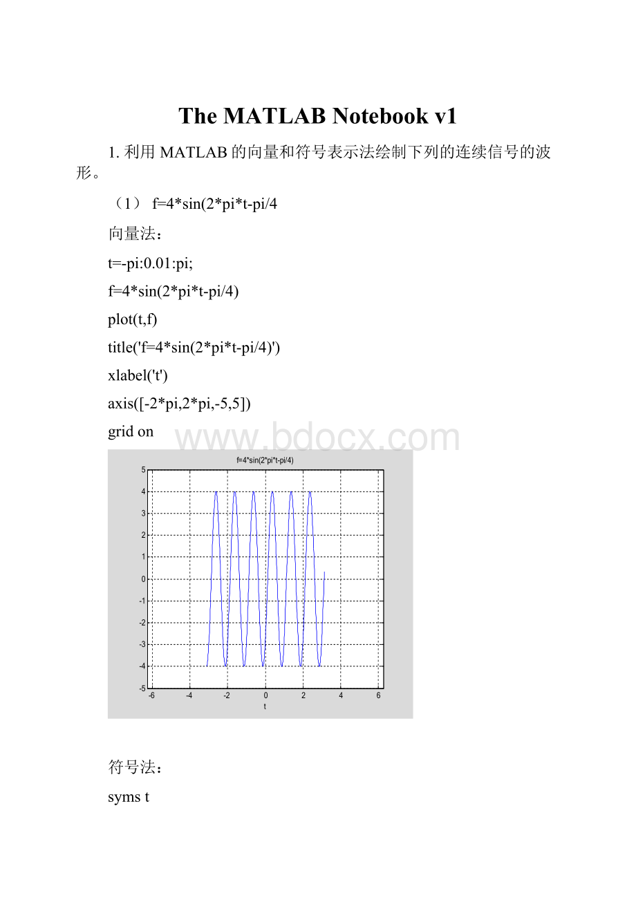
(1)f=4*sin(2*pi*t-pi/4
向量法:
t=-pi:
0.01:
pi;
f=4*sin(2*pi*t-pi/4)
plot(t,f)
title('f=4*sin(2*pi*t-pi/4)')
xlabel('t')
axis([-2*pi,2*pi,-5,5])
gridon
符号法:
symst
f=sym('4*sin(2*pi*t-pi/4)')
ezplot(f,[-2*pi,2*pi])
set(gcf,'color','w')
f=
4*sin(2*pi*t-pi/4)
2.f=(1-exp(-2*t))*u;
向量法
t=-6:
0.5:
6;
f=(1-exp(-2*t)).*Heaviside(t);
plot(t,f)
axis([-6,6,-0.3,1.2])
f=
Columns1through17
00000000000001111
Columns18through25
11111111
符号法:
symst;
f=sym('(1-exp(-2*t))*Heaviside(t)');
ezplot(f,[-5,5]);
3利用MATLAB绘制下列离散信号的波形
1.x(n)=cos(2*n/pi)*u(n)
n=-3:
6
u=jyxl(n);
stem(n,cos(n*pi/2).*u,'filled')
title('cos(n*pi/2).*u')
n=
-3-2-10123456
x=
0001111111
2
n=-6:
6;
u=jyxl(n);
f=jyxl(n-5);
stem(n,n.*(u-f),'filled')
title('n.*(u(n)-u(n-5)')
x=
0000001111111
x=
0000000000011
7.6已经知道连续时间信号f(t)=sin(pi*t/t),使用MATLAB编程绘制下列信号的波形
(1)、2*f(t-1)
symst
f=(sin(pi*t))/t;
f1=subs(f,t,t-1);
f2=2*f1;
ezplot(f2,[-3,3])
title('(sin(pi*(t-1)))/t')
axis([-3,3,-3,4])
(2)f(2*t)
symst
f=(sin(pi*t))/t;
f1=subs(f,t,2*t);
ezplot(f1,[-3,3])
title('f=(sin(pi*2*t))/t')
axis([-3,3,-3,4])
7.8使用MATLAB绘制下列复指数序列的实部、虚部、模和幅角随时间变化的波形图,观察分析副支书序列的时域特性。
(1)、x(n)=exp(j*n*pi)
n=-10:
10;
x=exp(i*n*pi);
Xr=real(x);
Xi=imag(x);
Xa=abs(x);
Xn=angle(x);
subplot(2,2,1),stem(n,Xr,'filled'),title('实部'),xlabel('n');
subplot(2,2,3),stem(n,Xi,'filled'),title('虚部');xlabel('n');
subplot(2,2,2),stem(n,Xa,'filled'),title('模');xlabel('n');
subplot(2,2,4),stem(n,Xn,'filled'),title('幅角');xlabel('n')
7.9
(1)x(-n-2)
x=[0,3,3,3,3,2,1,0,0];
n=-4:
4;
[x1,n1]=xlfz(x,n)
[x2,n2]=xlpy(x1,n1,-2)
stem(n2,x2,'filled')
x1=
001233330
n1=
-4-3-2-101234
x2=
001233330
n2=
-6-5-4-3-2-1012
(4)、x(n-4)x(n-2)
x1=[0,3,3,3,3,2,1,0,0];
n1=-4:
4;
[x2,n2]=xlpy(x1,n1,4)
x3=[0,3,3,3,3,2,1,0,0];
n3=-4:
4;
[x4,n4]=xlpy(x3,n3,2)
[x5,n5]=cxl(x2,x4,n2,n4)
stem(n5,x5,'filled')
x2=
033332100
n2=
012345678
x4=
033332100
n4=
-2-10123456
x5=
00099630000
n5=
-2-1012345678
7.10使用MATLAB生成并绘制额如下的信号波形
(1)、周期为2,峰值为5,的周期方波信号
t=0:
0.01:
10;
f=5*square(pi*t);
plot(t,f)
axis([-1,11,-6,6])
(2)、周期为PI,峰值为1的周期锯齿波
t=0:
0.01:
10;
f=sawtooth(2*t);
plot(t,f)
axis([0,10,-1.2,1.2])
 升级会员
升级会员 