信号的频谱图实验报告.docx
《信号的频谱图实验报告.docx》由会员分享,可在线阅读,更多相关《信号的频谱图实验报告.docx(15页珍藏版)》请在冰豆网上搜索。
信号的频谱图实验报告
大连理工大学实验报告
学院(系):
专业:
______________________班级:
___
姓名:
学号:
组:
___
实验时间:
实验室:
实验台:
指导教师签字:
成绩:
实验一信号的频谱图
一、实验目的
1.掌握周期信号的傅里叶级数展开
2.掌握周期信号的有限项傅里叶级数逼近
3.掌握周期信号的频谱分析
4.掌握连续非周期信号的傅立叶变换
5.掌握傅立叶变换的性质
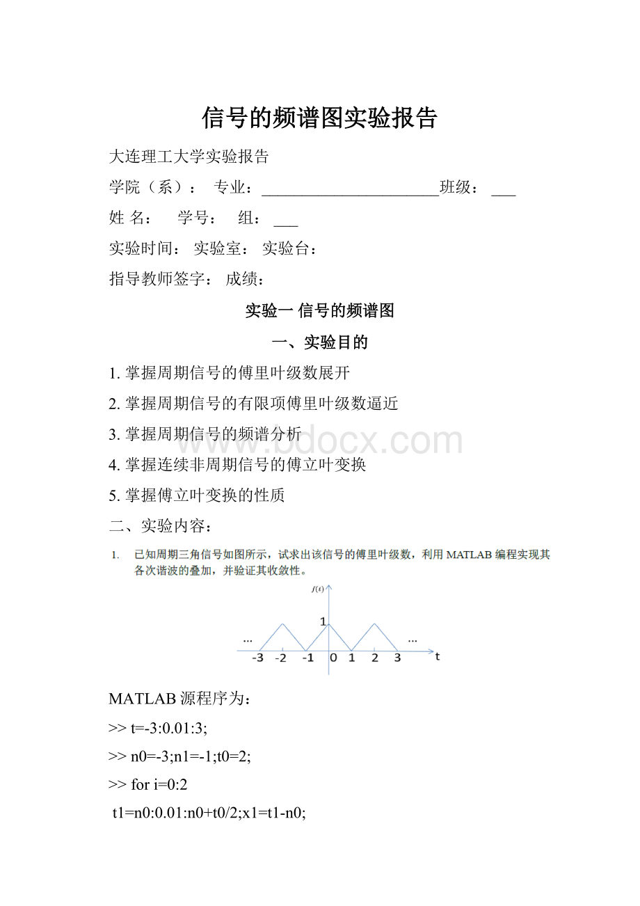
二、实验内容:
MATLAB源程序为:
>>t=-3:
0.01:
3;
>>n0=-3;n1=-1;t0=2;
>>fori=0:
2
t1=n0:
0.01:
n0+t0/2;x1=t1-n0;
t2=n1-t0/2:
0.01:
n1;x2=-t2+n1;
plot(t1,x1,'r',t2,x2,'r');
holdon;
n0=n0+t0;n1=n1+t0;
end
>>n_max=[1371531];
>>N=length(n_max);
>>fork=1:
N
n=1;sum=0;
while(n<(n_max(k)+1))
b=4./pi/pi/n/n;
y=b*cos(n*pi*t);
sum=sum+y;
n=n+2;
end
figure;
n0=-3;n1=-1;t0=2;
fori=0:
2
t1=n0:
0.01:
n0+t0/2;x1=t1-n0;
t2=n1-t0/2:
0.01:
n1;x2=-t2+n1;
plot(t1,x1,'r',t2,x2,'r');
holdon;
n0=n0+t0;n1=n1+t0;
end
y=sum+0.5;
plot(t,y,'b');
xlabel('t'),ylabel('wove');
holdoff;
axis([-3.013.01-0.011.01]);
gridon;
title(['themax=',num2str(n_max(k))])
end
运行结果:
MATLAB源程序为:
>>fork=1:
3;
n=-30:
30;tao=k;T=2*k;w=2*pi/T;
x=n*tao*0.5
fn1=sinc(x/pi);
fn=tao*fn1.*fn1;
subplot(3,1,k),stem(n*w,fn);
gridon
title(['T=',num2str(2*k)]);
axis([-30300k]);
end
运行结果:
x=
Columns1through9
-15.0000-14.5000-14.0000-13.5000-13.0000-12.5000-12.0000-11.5000-11.0000
Columns10through18
-10.5000-10.0000-9.5000-9.0000-8.5000-8.0000-7.5000-7.0000-6.5000
Columns19through27
-6.0000-5.5000-5.0000-4.5000-4.0000-3.5000-3.0000-2.5000-2.0000
Columns28through36
-1.5000-1.0000-0.500000.50001.00001.50002.00002.5000
Columns37through45
3.00003.50004.00004.50005.00005.50006.00006.50007.0000
Columns46through54
7.50008.00008.50009.00009.500010.000010.500011.000011.5000
Columns55through61
12.000012.500013.000013.500014.000014.500015.0000
x=
Columns1through16
-30-29-28-27-26-25-24-23-22-21-20-19-18-17-16-15
Columns17through32
-14-13-12-11-10-9-8-7-6-5-4-3-2-101
Columns33through48
234567891011121314151617
Columns49through61
18192021222324252627282930
x=
Columns1through9
-45.0000-43.5000-42.0000-40.5000-39.0000-37.5000-36.0000-34.5000-33.0000
Columns10through18
-31.5000-30.0000-28.5000-27.0000-25.5000-24.0000-22.5000-21.0000-19.5000
Columns19through27
-18.0000-16.5000-15.0000-13.5000-12.0000-10.5000-9.0000-7.5000-6.0000
Columns28through36
-4.5000-3.0000-1.500001.50003.00004.50006.00007.5000
Columns37through45
9.000010.500012.000013.500015.000016.500018.000019.500021.0000
Columns46through54
22.500024.000025.500027.000028.500030.000031.500033.000034.5000
Columns55through61
36.000037.500039.000040.500042.000043.500045.0000
MATLAB源程序为:
(1)>>ft=sym('sin(2*pi*(t-1))/(pi*(t-1))');
>>Fw=fourier(ft);
>>subplot(2,1,1);
>>ezplot(abs(Fw));
>>gridon;
>>title('fudupu');
>>phase=atan(imag(Fw)/real(Fw));
>>subplot(2,1,2);
>>ezplot(phase);
>>gridon;
>>title('xiangweipu');
运行结果:
(2)
MATLAB源程序为:
>>ft=sym('(sin(pi*t)/(pi*t))^2');
>>Fw=fourier(ft);
>>subplot(2,1,1);
>>ezplot(abs(Fw));
>>gridon;
>>title('fudupu');
>>phase=atan(imag(Fw)/real(Fw));
>>subplot(2,1,2);
>>ezplot(phase);
>>gridon;
>>title('xiangweipu');
运行结果:
(1)
MATLAB源程序为:
>>symst
>>Fw=sym('10/(3+i*w)-4/(5+i*w)')
Fw=
10/(w*i+3)-4/(w*i+5)
>>ft=ifourier(Fw,t)
ft=
(20*pi*exp(-3*t)*heaviside(t)-8*pi*exp(-5*t)*heaviside(t))/(2*pi)
>>ezplot(ft);
>>gridon;
运行结果:
(2)
MATLAB源程序为:
>>symst
>>Fw=sym('exp(-4*w^2)')
Fw=
exp(-4*w^2)
>>ft=ifourier(Fw,t)
ft=
exp(-t^2/16)/(4*pi^(1/2))
>>ezplot(ft);
>>gridon;
运行结果:
MATLAB源程序为:
>>dt=0.01;
>>t=-4:
dt:
4;
>>gt=(-1/2<=t&t<=1/2);
>>N=2000;
>>k=-N:
N;
>>W=2*pi*k/((2*N+1)*dt);
>>F=dt*gt*exp(-j*t'*W);
>>plot(W,F);
警告:
复数X和/或Y参数的虚部已忽略
>>gridon
>>xlabel('W'),ylabel('F(W)')
>>title('频谱图');
>>axis([-200200-0.251.1]);
运行结果:
MATLAB源程序为:
>>dt=0.01;
>>t=-0.6:
dt:
0.6;
>>f=rectpuls(t,1);
>>F=conv(f,f)*dt;n=length(F);
>>tt=(0:
n-1)*dt-1.2;
>>N=2000;k=-N:
N;
>>w=2*pi*k/((2*N+1)*dt);
>>fw=dt*f*exp(-j*t'*w);
>>FW=dt*F*exp(-j*tt'*w);
>>subplot(321),plot(t,f,'linewidth',2),gridon;
>>axis([-0.7,0.7,-0.1,1.1]);
>>title('f');%门信号图形
>>subplot(322),plot(w,fw,'linewidth',2),gridon;
警告:
复数X和/或Y参数的虚部已忽略
>>axis([-20,20,-0.5,1.1]);
>>title('fw');%门信号频谱图
>>subplot(323),plot(tt,F,'linewidth',2),gridon;
>>axis([-1.3,1.3,-0.2,1.2]);
>>title('f*f');%两门信号卷积的图形
>>subplot(324),plot(w,fw.*fw,'linewidth',2),gridon;
警告:
复数X和/或Y参数的虚部已忽略
>>axis([-20,20,-0.1,1.1]);
>>title('fw*fw');%门信号频域相乘的图形
>>subplot(326),plot(w,FW,'linewidth',2),gridon;
警告:
复数X和/或Y参数的虚部已忽略
>>axis([-20,20,-0.1,1.1]);
>>title('Fourier(f*f)');%两门信号卷积,再Fourier变换
>>
运行结果:
由于两门信号卷积的图形与两门信号卷积再傅里叶变换的图形基本一致,所以傅里叶变换的时域卷积定理得证。
三、实验体会
这是第一次信号上机实验,在这次实验中第一次接触到了MATLAB这个工程软件,MATLAB功能强大,操作相对简单。
同时本节课中我学会了对绘制信号的时域波形和对信号进行频域分析。
通过MATLAB可以非常直观的看到了,信号的叠加合成等现象。
 升级会员
升级会员 