R软件 主成分分析文档格式.docx
《R软件 主成分分析文档格式.docx》由会员分享,可在线阅读,更多相关《R软件 主成分分析文档格式.docx(14页珍藏版)》请在冰豆网上搜索。
48.287
0.386
14.5
25.9
23.32
2.18
0.93
6
17.956
0.28
9.75
17.05
37.2
0.464
7
7.37
0.506
13.6
34.28
10.69
8.8
0.56
8
4.223
0.34
3.8
7.1
88.2
1.11
0.97
9
6.442
0.19
4.7
9.1
73.2
0.74
1.03
10
16.234
0.39
3.1
5.4
121.5
0.42
1.0
11
10.585
2.4
135.6
0.87
12
23.535
0.23
2.6
4.6
151.8
0.31
1.02
13
5.398
0.12
2.8
6.2
111.2
1.14
1.07
14
283.149
0.148
1.763
2.968
215.86
0.14
15
316.604
0.317
1.453
2.432
263.41
0.249
16
307.31
0.173
1.627
2.729
235.7
0.214
0.99
17
322.515
0.312
1.382
2.32
282.21
0.024
1.00
18
254.58
0.297
0.899
1.476
410.3
0.239
19
304.092
0.283
0.789
1.357
438.36
0.193
20
202.446
0.042
0.741
1.266
309.77
0.29
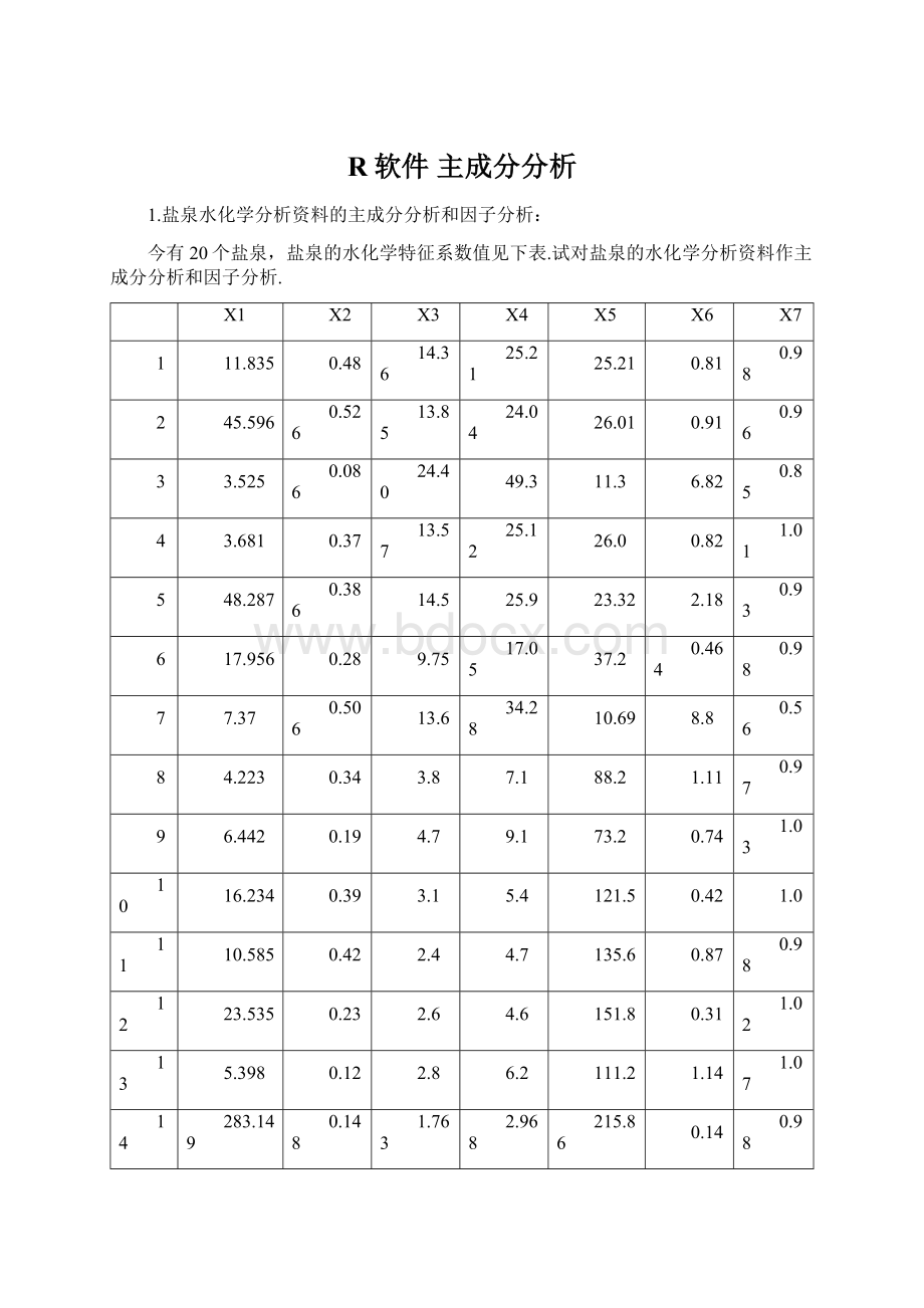
其中x1:
矿化度(g/L);
x2:
Br•103/Cl;
x3:
K•103/Σ盐;
x4:
K•103/Cl;
x5:
Na/K;
x6:
Mg•102/Cl;
x7:
εNa/εCl.
1.数据准备
导入数据保存在对象saltwell中
>
saltwell<
-read.table("
c:
/saltwell.txt"
header=T)
saltwell
X1X2X3X4X5X6X7
111.8350.48014.36025.21025.210.8100.98
245.5960.52613.85024.04026.010.9100.96
33.5250.08624.40049.30011.306.8200.85
43.6810.37013.57025.12026.000.8201.01
548.2870.38614.50025.90023.322.1800.93
617.9560.2809.75017.05037.200.4640.98
77.3700.50613.60034.28010.698.8000.56
84.2230.3403.8007.10088.201.1100.97
96.4420.1904.7009.10073.200.7401.03
1016.2340.3903.1005.400121.500.4201.00
1110.5850.4202.4004.700135.600.8700.98
1223.5350.2302.6004.600151.800.3101.02
135.3980.1202.8006.200111.201.1401.07
14283.1490.1481.7632.968215.860.1400.98
15316.6040.3171.4532.432263.410.2490.98
16307.3100.1731.6272.729235.700.2140.99
17322.5150.3121.3822.320282.210.0241.00
18254.5800.2970.8991.476410.300.2390.93
19304.0920.2830.7891.357438.360.1931.01
20202.4460.0420.7411.266309.770.2900.99
2.数据分析
1标准误、方差贡献率和累积贡献率
arrests.pr<
-prcomp(saltwell,scale=TRUE)
summary(arrests.pr,loadings=TRUE)
Importanceofcomponents:
PC1PC2PC3PC4PC5PC6PC7
Standarddeviation2.06081.11750.95920.661530.338410.177280.02614
ProportionofVariance0.60670.17840.13140.062520.016360.004490.00010
CumulativeProportion0.60670.78510.91650.979050.995410.999901.00000
2每个变量的标准误和变换矩阵
prcomp(saltwell,scale=TRUE)
Standarddeviations:
[1]2.06081091.11746860.95919800.66153460.33841220.17727720.0261419
Rotation:
PC1PC2PC3PC4PC5PC6
X10.34688530.504503850.04884241-0.55817600.5239549-0.191489310
X2-0.2002213-0.120290250.93023876-0.1733966-0.0967612-0.201658411
X3-0.4414777-0.05850625-0.18016824-0.5534399-0.15360550.186904467
X4-0.45860100.04257557-0.18275574-0.4025103-0.14823750.009825109
X50.40560060.417668390.04962230-0.1398811-0.79545970.079036986
X6-0.40063530.44480041-0.138996850.2887128-0.1012846-0.709580413
X70.3306722-0.59453862-0.21125225-0.2951966-0.1659059-0.614723279
PC7
X1-0.001864597
X2-0.001522652
X30.635916793
X4-0.755239886
X5-0.003042766
X60.158763393
X7-0.001295549
3查看对象arests.pr中的内容
>
str(arrests.pr)
Listof5
$sdev:
num[1:
7]2.0611.1170.9590.6620.338...
$rotation:
7,1:
7]0.347-0.2-0.441-0.4590.406...
..-attr(*,"
dimnames"
)=Listof2
....$:
chr[1:
7]"
X1"
"
X2"
X3"
X4"
...
PC1"
PC2"
PC3"
PC4"
$center:
Namednum[1:
7]109.7680.2956.60412.627149.842...
names"
)=chr[1:
$scale:
7]134.1890.1386.78113.572134.642...
$x:
20,1:
7]-1.67-1.66-4.1-1.39-1.88...
NULL
-attr(*,"
class"
)=chr"
prcomp"
4利用主成分的标准误计算出主成分的累积方差比例
cumsum(arrests.pr$sdev^2)/7
[1]0.60670600.78509680.91653410.97905240.99541280.99990241.0000000
5各个化学成分占主成分的得分
arrests.pr$x
PC1PC2PC3PC4PC5
[1,]-1.67419700-1.15390757.812973e-01-0.82154434-0.09559387
[2,]-1.65924015-0.93029891.166840e+00-0.874901520.05107312
[3,]-4.098385481.0111567-2.567612e+00-0.68730247-0.31976517
[4,]-1.38589039-1.24908033.749759e-05-0.66715185-0.08448647
[5,]-1.88022254-0.38899371.671917e-01-0.571127580.13190861
[6,]-0.69655135-0.9728592-3.030663e-01-0.034241970.20614983
[7,]-4.753206462.74264371.213314e+001.168467300.18776151
[8,]-0.08633651-0.71588223.871693e-010.785116490.04007332
[9,]0.22003394-1.0391225-7.757745e-010.630159110.12089601
[10,]0.29149770-0.91519367.624748e-010.57357593-0.12752807
[11,]0.20307566-0.71352461.008511e+000.73605261-0.21843357
[12,]0.77537521-0.7882670-3.089778e-010.70624777-0.17305749
[13,]0.71166897-1.0074449-1.248452e+000.86096256-0.06535513
[14,]1.770617670.6549572-6.064948e-01-0.128936570.62744865
[15,]1.775069430.80349935.680314e-01-0.474313490.36704946
[16,]1.892374560.7433814-4.402613e-01-0.282171090.57360330
[17,]1.965394110.73093015.200281e-01-0.588025960.26351255
[18,]1.997721491.32828585.946532e-01-0.13000624-0.62597984
[19,]2.503422741.14914743.741488e-01-0.56734140-0.71010526
[20,]2.127778380.7105729-1.293059e+000.36648272-0.14917150
PC6PC7
[1,]0.07084792-0.007513416
[2,]0.028143710.015953231
[3,]-0.152160160.016299237
[4,]0.04143780-0.074960637
[5,]0.029513800.063346130
[6,]0.33477919-0.007866628
[7,]0.01788053-0.024497758
[8,]-0.015429830.031130241
[9,]-0.02170366-0.020193011
[10,]-0.069563050.010431127
[11,]-0.138202810.014603566
[12,]0.072751440.001164613
[13,]-0.31007297-0.009840824
[14,]0.12358561-0.001945118
[15,]-0.185193610.002965969
[16,]-0.021469220.002545690
[17,]-0.22556715-0.013751662
[18,]0.300591020.001904014
[19,]-0.19369360-0.007138842
[20,]0.313525040.007364079
5.数据分析结果图形表示
screeplot(arrests.pr,main="
saltwell"
)
biplot(arrests.pr)
按第一主成分排序的结果:
data.frame(sort(arrests.pr$x[,1]))
sort.arrests.pr.x...1..
1-4.75320646
2-4.09838548
3-1.88022254
4-1.67419700
5-1.65924015
6-1.38589039
7-0.69655135
8-0.08633651
90.20307566
100.22003394
110.29149770
120.71166897
130.77537521
141.77061767
151.77506943
161.89237456
171.96539411
181.99772149
192.12777838
202.50342274
主因子分析
计算数据的相关系数矩阵
saltwell.cor<
-cor(saltwell)
saltwell.cor
X11.0000000-0.2911815-0.5704925-0.56763260.8488512-0.38857440.1689518
X2-0.29118151.00000000.27250120.2592747-0.34623270.1386043-0.3445447
X3-0.57049250.27250121.00000000.9868546-0.75087730.6694637-0.4707286
X4-0.56763260.25927470.98685461.0000000-0.73793670.7778797-0.5854959
X50.8488512-0.3462327-0.7508773-0.73793671.0000000-0.47468580.2815300
X6-0.38857440.13860430.66946370.7778797-0.47468581.0000000-0.8875089
X70.1689518-0.3445447-0.4707286-0.58549590.2815300-0.88750891.0000000
计算特征值和特征向量及因子的贡献率和累积贡献率
saltwell.eigen<
-eigen(saltwell.cor)
saltwell.eigen
$values
[1]4.24694166751.24873605500.92006075820.43762806380.11452284400.03142721240.0006833991
$vectors
[,1][,2][,3][,4][,5][,6][,7]
[1,]0.3468853-0.504503850.04884241-0.55817600.5239549-0.191489310-0.001864597
[2,]-0.20022130.120290250.93023876-0.1733966-0.0967612-0.201658411-0.001522652
[3,]-0.44147770.05850625-0.18016824-0.5534399-0.15360550.1869044670.635916793
[4,]-0.4586010-0.04257557-0.18275574-0.4025103-0.14823750.009825109-0.755239886
[5,]0.4056006-0.417668390.04962230-0.1398811-0.79545970.079036986-0.003042766
[6,]-0.4006353-0.44480041-0.138996850.2887128-0.1012846-0.7095804130.158763393
[7,]0.33067220.59453862-0.21125225-0.2951966-0.1659059-0.614723279-0.001295549
根据主成分分析结果确定公共因子个数.
saltwell.pr<
-princomp(saltwell,cor=T)
summary(saltwell.pr)
Comp.1Comp.2Comp.3Comp.4Comp.5Comp.6Comp.7
Standarddeviation2.0608111.11746860.95919800.661534630.338412240.1772772192.614190e-02
ProportionofVariance0.6067060.17839090.13143730.062518290.016360410.0044896029.762844e-05
CumulativeProportion0.6067060.78509680.91653410.979052360.995412770.9999023721.000000e+00
均值
saltwell.pr$center
X1X2X3X4X5X6X7
109.768150.294806.6042012.62740149.842001.337150.96100
标准误
saltwell.pr$scale
130.79077540.13488726.609676913.2284214131.23287272.23307450.1016317
下面用特征值的平方根乘以相应的特征向量得到因子载荷矩阵.并且只显示前2个因子的结果:
t(sqrt(saltwell.eigen$values)*t(saltwell.eigen$vectors))[,1:
2]
[,1][,2]
[1,]0.7148649-0.56376721
[2,]-0.41261820.13442058
[3,]-0.90980210.06537890
[4,]-0.9450901-0.04757686
[5,]0.8358661-0.46673130
[6,]-0.8256336-0.49705049
[7,]0.68145290.66437824
用R语言自带的函数factanal()进行分析
saltwell.fa<
-factanal(saltwell,factors=2)
print(saltwell.fa,cutoff=0.001)
Call:
factanal(x=saltwell,factors=2)
Uniquenesses:
0.6680.9230.0050.0050.4280.0050.179
Loadings:
Factor1Factor2
X1-0.543-0.193
X20.2730.045
X30.9400.338
X40.8750.481
X5-0.725-0.213
X60.3820.922
X7-0.181-0.888
SSloadings2.7232.067
ProportionVar0.3890.295
CumulativeVar0.3890.684
Testofthehypothesisthat2factorsaresufficient.
Thechisquarestatisticis42.91on8degreesoffreedom.
Thep-valueis9.14e-0
 升级会员
升级会员 