Multiple Linear Regression Model1Word格式.docx

Multiple Linear Regression Model1Word格式.docx

《Multiple Linear Regression Model1Word格式.docx》由会员分享，可在线阅读，更多相关《Multiple Linear Regression Model1Word格式.docx（12页珍藏版）》请在冰豆网上搜索。

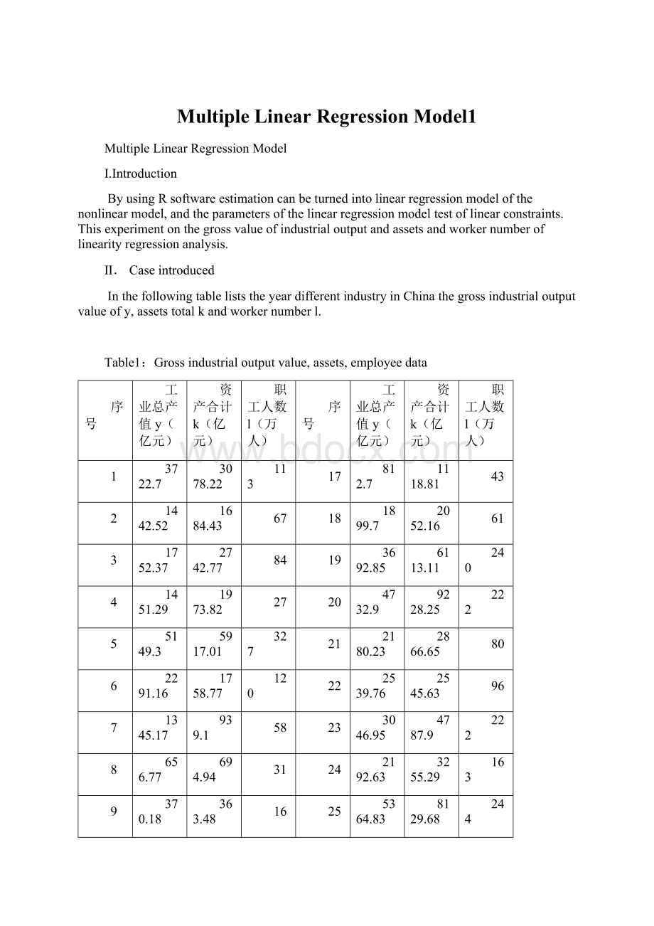
240

4

1451.29

1973.82

27

20

4732.9

9228.25

222

5

5149.3

5917.01

327

21

2180.23

2866.65

80

6

2291.16

1758.77

120

22

2539.76

2545.63

96

7

1345.17

939.1

58

23

3046.95

4787.9

8

656.77

694.94

31

24

2192.63

3255.29

163

9

370.18

363.48

16

25

5364.83

8129.68

244

10

1590.36

2511.99

66

26

4834.68

5260.2

145

11

616.71

973.73

7549.58

7518.79

138

12

617.94

516.01

28

867.91

984.52

46

13

4429.19

3785.91

29

4611.39

18626.94

218

14

5749.02

8688.03

254

30

170.3

610.91

15

1781.37

2798.9

83

325.53

1523.19

45

1243.07

1808.44

33

Ⅲ．ModelBuilding

3.1．Model_1Setamodelfor

Step1：

Readthedata

>

da=read.table（"

C:

/23/f.csv"

sep="

"

）

y=da[,2]

k=da[,3]

l=da[,4]

win.graph（width=3.5,height=3.5,pointsize=8）

plot（y,k）#plotthescatterofyandk

plot（y,l）#plotthescatterofyandl

Step2:

PARAMETERESTIMATION

m1=lm（y~k+l）

summary（m1）

Call:

lm（formula=y~k+l）

Residuals:

Min1QMedian3QMax

-2113.0-472.9-232.7196.53928.2

Coefficients:

EstimateStd.ErrortvaluePr（>

|t|）

（Intercept）588.61734339.389361.7340.09386.

k0.199260.081942.4320.02167*

l11.120213.622673.0700.00473**

---

Signif.codes:

0‘***’0.001‘**’0.01‘*’0.05‘.’0.1‘’1

Residualstandarderror:

1143on28degreesoffreedom

MultipleR-squared:

0.6715,AdjustedR-squared:

0.648

F-statistic:

28.62on2and28DF,p-value:

1.706e-07

Itisconcludedthatthefollowingregressionequation:

Analysisofvariance

anova（m1）

AnalysisofVarianceTable

Response:

y

DfSumSqMeanSqFvaluePr（>

F）

k1624666966246669647.80771.624e-07***

l112311730123117309.42250.004725**

Residuals28365854951306625

Residualanalysis

re1=residuals（m1）

plot（re1）

Step3：

Resultsanalysis

1.coefficientofdetermination

BecauseofR^2=0.6715,sothefittingeffectisnotgood

2．TESTSOFHYPOTHESES

Agivenlevelofsignificance:

qf（0.975,2,27）

[1]4.242094

qt（0.975,27）

[1]2.051831

F=28.62>

F（2,27）=4.24

P=1.706e-07<

0.05,Showthatk,lcombinedtohaveasignificantlinearimpactony.

T（k）=2.432〉t（27）=2.05；

T（l）=3.070〉t（27）=2.05，Showthatk,lofyhassignificantlinearinfluence.

3.Accordingtotheresidualfigure,wecanfindthatasthedatasequence,residualobviousdeviationfromthemean,theincreasescope,showedthatpoorregressionresults.

4.Theregressionequationresidualanalysis

plot（m1）

Fromtheaboveknowable,deviatingfromthefittinglinesituationisrelativelyserious,canalsobeconcludedthatthefittingeffectisnotgood.

3.2.Model2

Setamodelfor

Thelogarithmictransformation,

Canbeconvertedinto

Step1:

DATAPROCESSING

y1=log（y）#takelogarithms

k1=log（k）

l1=log（l）

Table2：

data（ln）

Serialnumber

Grossvalueofindustrialoutput

lnY

Assetstotal

lnK

Theworkernumber

lnL

（亿元）

（万人）

8.222204

8.032107

4.727388

7.274147

7.429183

4.204693

7.468724

7.916724

4.430817

7.280208

7.587726

3.295837

8.546616

8.685587

5.78996

7.736814

7.47237

4.787492

7.204276

6.844922

4.060443

6.487334

6.543826

3.433987

5.913989

5.895724

2.772589

7.371716

7.828831

4.189655

6.424399

6.881134

6.426391

6.246126

3.332205

8.395972

8.239042

4.110874

8.656785

9.069701

5.537334

7.485138

7.936982

4.418841

7.125339

7.50022

3.496508

6.700362

7.020021

3.7612

7.549451

7.626648

8.214154

8.718191

5.480639

8.462293

9.130025

5.402677

7.687186

7.960899

4.382027

7.839825

7.842133

4.564348

8.021896

8.473847

7.692857

8.088037

5.09375

8.58762

9.003277

5.497168

8.48357

8.567924

4.976734

8.929247

8.92516

4.927254

6.766088

6.892154

3.828641

8.436285

9.832364

5.384495

5.137562

6.41495

2.944439

5.785455

7.328562

3.806662

Parameterestimation

m2=lm（log（y）~log（k）+log（l））

summary（m2）

lm（formula=log（y）~log（k）+log（l））

-1.20679-0.155170.031790.265320.73927

（Intercept）1.15400.72761.5860.12397

log（k）0.60920.17643.4540.00178**

log（l）0.36080.20161.7900.08432.

0.4255on28degreesoffreedom

0.8099,AdjustedR-squared:

0.7963

59.66on2and28DF,p-value:

8.035e-11

（exp（1.1540）=3.170851）

anova（m2）

log（y）

log（k）121.024921.0249116.10691.805e-11***

log（l）10.58000.58003.20320.08432.

Residuals285.07030.1811

Residualanalysis

re2=residuals（m2）

plot（re2）

2.coefficientofdetermination

：

BecauseofR^2=0.8099，Sothefittingeffectisbetterthanmodel1.

3.TESTSOFHYPOTHESES

Agivenlevelofsignificanceis5%，

F=59.66>

P=8.035e-11<

0.05,ShowthatLNK,LNLcombinedtohaveasignificantlinearimpactonlny

。

T（lnk）=3.454>

2.05，T（lnl）=1.790<

2.05,LNKparametersthroughthetestofsignificanceofvariables;

ButtheparametersoftheLNLfailedtheinspection.

Ifagiven10%significancelevel

qt（0.95,27）

[1]1.703288

1.70;

T（lnl）=1.790>

1.70,SotheLNK,LNLparametersthroughthetestofsignificanceofvariables.

3.Accordingtotheresidualfigure,wecanfindthatinadditiontothethreeabnormalpointsafter,evenlydistributedaroundthezeroresidual,andvolatility,within0.5regressionresultisgood.

4.Theregressionequationresidualfigure

plot（m2）