统计建模与R软件（薛毅）第九章答案Word文档下载推荐.doc

统计建模与R软件（薛毅）第九章答案Word文档下载推荐.doc

《统计建模与R软件（薛毅）第九章答案Word文档下载推荐.doc》由会员分享，可在线阅读，更多相关《统计建模与R软件（薛毅）第九章答案Word文档下载推荐.doc（12页珍藏版）》请在冰豆网上搜索。

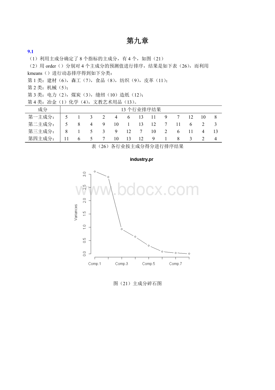
第一主成分：

5

1

3

2

4

6

13

11

9

7

12

10

8

第二主成分：

第三主成分：

第四主成分：

表（26）各行业按主成分得分进行排序结果

图（21）主成分碎石图

图（22）第一主成分与第二主成分下的散点图

习题程序与结论：

>

industry<

-data.frame（

+X1=c（90342,4903,6735,49454,139190,12215,2372,11062,17111,1206,2150,5251,14341），

+X2=c（52455,1973,21139,36241,203505,16219,6572,23078,23907,3930,5704,6155,13203），

+X3=c（101091,2035,3767,81557,215898,10351,8103,54935,52108,6126,6200,10383,19396）,

+X4=c（19272,10313,1780,22504,10609,6382,12329,23804,21796,15586,10870,16875,14691）,

+X5=c（82.0,34.2,36.1,98.1,93.2,62.5,184.4,370.4,221.5,330.4,184.2,146.4,94.6）,

+X6=c（16.1,7.1,8.2,25.9,12.6,8.7,22.2,41.0,21.5,29.5,12.0,27.5,17.8）,

+X7=c（197435,592077,726396,348226,139572,145818,20921,65486,63806,1840,8913,78796,6354）,

+X8=c（0.172,0.003,0.003,0.985,0.628,0.066,0.152,0.263,0.276,0.437,0.274,0.151,1.574））

industry.pr<

-princomp（industry,cor=T）

summary（industry.pr）####做主成分分析，得到4个主成分，累积贡献率达94.68%

Importanceofcomponents:

Comp.1Comp.2Comp.3Comp.4Comp.5

Standarddeviation1.76207621.70218730.96447680.801325320.55143824

ProportionofVariance0.38811410.36218020.11627690.080265280.03801052

CumulativeProportion0.38811410.75029430.86657120.946836490.98484701

Comp.6Comp.7Comp.8

Standarddeviation0.294274970.1794000620.0494143207

ProportionofVariance0.010824720.0040230480.0003052219

CumulativeProportion0.995671730.9996947781.0000000000

load<

-loadings（industry.pr）####求出载荷矩阵

load

Loadings:

Comp.1Comp.2Comp.3Comp.4Comp.5Comp.6Comp.7Comp.8

X1-0.477-0.296-0.1040.1840.7580.245

X2-0.473-0.278-0.163-0.174-0.305-0.5180.527

X3-0.424-0.378-0.156-0.174-0.781

X40.213-0.4510.5160.5390.288-0.2490.220

X50.388-0.331-0.321-0.199-0.4500.5820.233

X60.352-0.403-0.1450.279-0.317-0.714

X7-0.2150.377-0.1400.758-0.4180.194

X8-0.2730.891-0.3220.122

Comp.1Comp.2Comp.3Comp.4Comp.5Comp.6Comp.7Comp.8

SSloadings1.0001.0001.0001.0001.0001.0001.0001.000

ProportionVar0.1250.1250.1250.1250.1250.1250.1250.125

CumulativeVar0.1250.2500.3750.5000.6250.7500.8751.000

plot（load[,1:

2]）

text（load[,1],load[,2],adj=c（-0.4,-0.3））

screeplot（industry.pr,npcs=4,type="

lines"

）####得出主成分的碎石图

biplot（industry.pr）####得出在第一，第二主成分之下的散点图

p<

-predict（industry.pr）####预测数据，讲预测值放入p中

order（p[,1]）;

order（p[,2]）;

order（p[,3]）;

order（p[,4]）;

####将预测值分别以第一，第二，第三，第四主成分进行排序

[1]51324613119712108

[1]58491011312711623

[1]81539127102611413

[1]11657101312918324

kmeans（scale（p）,4）####将预测值进行标准化，并分为4类

K-meansclusteringwith4clustersofsizes5,1,4,3

Clustermeans:

Comp.1Comp.2Comp.3Comp.4Comp.5Comp.6

10.5132590-0.03438438-0.3405983-0.51300310.23551510.22441040

2-2.5699693-1.32913757-0.4848689-0.9460127-0.9000187-0.06497950

30.23815810.72871986-0.29959180.3126036-0.4744091-0.19709710

4-0.3163193-0.471273331.12874260.75353800.5400265-0.08956137

Comp.7Comp.8

1-0.38197798-0.7474855

2-0.675002090.4569548

30.090630690.9826915

40.74078975-0.2167643

Clusteringvector:

[1]4334211113134

Withinclustersumofsquaresbycluster:

[1]19.411370.0000024.4950416.61172

（between_SS/total_SS=37.0%）

Availablecomponents:

[1]"

cluster"

"

centers"

totss"

"

withinss"

"

tot.withinss"

[6]"

betweenss"

"

size"

9.2

####用数据框的形式输入数据

sale<

X1=c（82.9,88.0,99.9,105.3,117.7,131.0,148.2,161.8,174.2,184.7）,

X2=c（92,93,96,94,100,101,105,112,112,112）,

X3=c（17.1,21.3,25.1,29.0,34.0,40.0,44.0,49.0,51.0,53.0）,

X4=c（94,96,97,97,100,101,104,109,111,111）,

Y=c（8.4,9.6,10.4,11.4,12.2,14.2,15.8,17.9,19.6,20.8）

）

####作线性回归

lm.sol<

-lm（Y~X1+X2+X3+X4,data=sale）

summary（lm.sol）

显示结果

Call:

lm（formula=Y~X1+X2+X3+X4,data=sale）

Residuals:

1234567

0.0248030.0794760.012381-0.007025-0.2883450.216090-0.142085

8910

0.158360-0.1359640.082310

Coefficients:

EstimateStd.ErrortvaluePr（>

|t|）

（Intercept）-17.667685.94360-2.9730.03107*

X1