有序分类资料的统计分析Stata实现.docx
《有序分类资料的统计分析Stata实现.docx》由会员分享,可在线阅读,更多相关《有序分类资料的统计分析Stata实现.docx(17页珍藏版)》请在冰豆网上搜索。
有序分类资料的统计分析Stata实现
第十二章有序分类资料的统计分析的Stata实现
本章使用的STATA命令:
列变量有序时的分类资料CMH卡方分析
opartchi行变量[weight],by(列变量)
(见Stata7附加程序)
双向有序时的Spearman相关
spearman变量1变量2
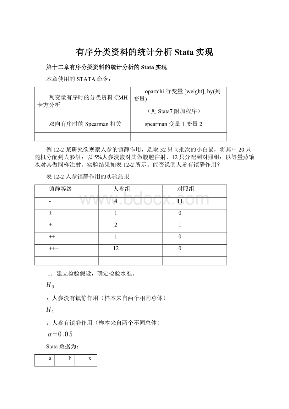
例12-2某研究欲观察人参的镇静作用,选取32只同批次的小白鼠,将其中20只随机分配到人参组:
以5%人参浸液对其做腹腔注射,12只分配到对照组:
以等量蒸馏水对其做同样注射。
实验结果如表12-2所示。
能否说明人参有镇静作用?
表12-2人参镇静作用的实验结果
镇静等级
人参组
对照组
-
4
11
±
1
0
+
2
1
++
1
0
+++
12
0
1.建立检验假设,确定检验水准。
:
人参没有镇静作用(样本来自两个相同总体)
:
人参有镇静作用(样本来自两个不同总体)
Stata数据为:
a
b
x
1
1
4
1
2
1
1
3
2
1
4
1
1
5
12
2
1
11
2
2
0
2
3
1
2
4
0
2
5
0
Stata命令为:
opartchib[weight=x],by(a)
结果为:
Chi-squaretests
dfChi-squareP-value
Independence416.640.0023
-------------------------------------------------------
Componentsofindependencetest
Location115.290.0001
Dispersion1.34960.5543
在
的水平上,拒绝
,接受H1,认为两总体之间的差别有统计学意义,可以认为人参组和对照组镇静等级的差别有统计学意义,人参有镇静作用。
例12-3试根据表12-4的资料,检验针刺不同穴位的镇痛效果有无差别?
表12-4针刺不同穴位的镇痛效果
穴位
镇痛效果
+
++
+++
++++
合谷
38
44
12
24
足三里
53
29
28
16
扶突
47
23
19
33
1.建立检验假设,确定检验水准。
:
三个穴位的镇痛效果相同
:
三个穴位的镇痛效果不全相同
Stata数据为:
group
effect
w
1
1
38
1
2
44
1
3
12
1
4
24
2
1
53
2
2
29
2
3
28
2
4
16
3
1
47
3
2
23
3
3
19
3
4
33
Stata命令为:
opartchieffect[weight=w],by(group)
结果为:
Chi-squaretests
dfChi-squareP-value
Independence622.070.0012
-------------------------------------------------------
Componentsofindependencetest
Location23.1180.2103
Dispersion25.9140.0520
有
。
在
的水平上尚不能拒绝
,即根据本例资料尚不能认为针刺不同穴位的镇痛效果差别有统计学意义。
例12-4两名放射科医师对13张肺部X线片各自做出评定,评定方法是将X线片按病情严重程度给出等级,结果如表12-6所示。
问他们的评定结果是否相关。
表12-6两名放射科医师对13张肺部X片的评定结果
X片编号
1
2
3
4
5
6
7
8
9
10
11
12
13
甲医师X
+
++
-
-
+
++
+++
++
+++
-
++
+
乙医师Y
++
+
+
-
++
+++
++
+++
+++
++
++
1.建立检验假设,确定检验水准。
:
=0(两名医师的等级评定结果不相关)
:
(两名医师的等级评定结果相关)
Stata数据为:
i
x
y
1
2
1
2
3
3
3
0
2
4
1
2
5
0
0
6
2
3
7
3
4
8
4
3
9
3
4
10
4
4
11
0
1
12
3
3
13
2
3
Stata命令为:
spearmanyx
结果为:
Numberofobs=13
Spearman'srho=0.8082
TestofHo:
yandxareindependent
Prob>|t|=0.0008
P<0.05。
在
水平上,拒绝H0,接受H1,认为两名射科医师对肺部X片的等级评定结果有正相关关系。
例12-5300名抑郁症患者按其抑郁程度和自杀意向的轻重程度的分类数据如表12-8所示。
问自杀意向的轻重程度和抑郁程度之间是否存在线性变化趋势?
表12-8300名抑郁症患者的分类数据
自杀意向(X)
抑郁程度(Y)
合计
轻度
中等
严重
(Y=1)
(Y=2)
(Y=3)
无
(X=1)
135
73
14
222
想要自杀
(X=2)
5
9
10
24
曾自杀过
(X=3)
8
23
23
54
合计
148
105
47
300
1、建立检验假设,确定检验水准。
:
自杀意向与抑郁症之间不存在线性变化趋势
:
自杀意向与抑郁症之间存在线性变化趋势
Stata数据为:
y
x
w
1
1
135
1
2
5
1
3
8
2
1
73
2
2
9
2
3
23
3
1
14
3
2
10
3
3
23
Stata命令和结果为*:
.corryx[fw=w]
(obs=300)
|yx
-------------+------------------
y|1.0000
x|0.46421.0000
.returnlist
scalars:
r(N)=300
r(rho)=.4641844307421609
.display(r(N)-1)*r(rho)^2
64.424689
在
水平上,拒绝H0,接受H1,可以推断自杀意向的轻重程度与抑郁症之间存在线性变化趋势。
*参考文献:
DoesStataprovideatestfortrend?
Title
Acomparisonofdifferenttestsfortrend
Author
WilliamSribney,StataCorp
Date
March1996
LetmemakeabunchofcommentscomparingSASPROCFREQ,Pearson’scorrelation,PatrickRoyston’sptrendcommand,linearregression,logit/probitregression,Stata’svwlscommand,andStata’snptrendcommand.
Testsfortrendin2xrtables
LetmeuseLesKalish’sexample:
Outcome
----------------------------
group|Good|Better|Best
y_i|a_1=1|a_2=2|a_3=3
------+--------+--------+---------
|||
y_1=0|19|31|67
|n_11|n_12|n_13
|||
y_2=1|1|5|21
|n_21|n_22|n_23
|||
------+--------+--------+---------
203688
n_+1n_+2n_+3
PROCFREQ
WhenIusedSASingradschooltoanalyzethesedata,weused
PR0CFREQDATA=...
TABLESGROUP*OUTCOME/CHISQCMHSCORES=TABLE
Theteststatisticwasshownontheoutputas
DFValueProb
-------------
Mantel-HaenszelChi-Square14.5150.034
TheteststatisticisnotaMantel–Haenszel—atleastnotaccordingtowhatIlearnedaMantel–Haenszelstatisticis(fromGaryKochatUNC—notethatanyerrorshere,Ishouldadd,arethoseofthisstudent,notofthisgreatresearcher/teacher).
Dr.Kochcalledthischi-squaredstatisticQs,wheresstandsforscore.
Chi-squaredstatisticfortrendQs
LetmeexpressQsintermsofasimplerstatistic,T:
T=(sumovergroupi)(sumoveroutcomej)nij*aj*yi
Theajarescores;here1,2,3,buttherecanbeotherchoicesforthescores(I’llgettothislater).
Underthenullhypothesisthereisnoassociationbetweengroupandoutcome,sowecanconsiderthepermutation(i.e.,randomization)distributionofT.Thatis,wefixthemarginsofthetable,justaswedoforFisher’sexacttest,andthenconsiderallthepossiblepermutationsthatgivethesesamemarginalcounts.
Underthisnullhypothesispermutationdistribution,itiseasytoseethatthemeanofTis
E(T)=N*a_bar*y_bar
wherea_baristheweightedaverageofaj(usingthemarginalcountsn+j):
a_bar=(sumoverj)n+j*aj/N
Similarly,y_barisaweightedaverageofyi.
ThevarianceofT,underthepermutationdistribution,is(exactly)
V(T)=(N-1)*Sa2*Sy2
whereSa2isthestandarddeviationsquaredforaj:
Sa2=(1/(N-1))*(sumoverj)n+j*(aj-a_bar)2
Wecancomputeachi-squaredstatistic:
Qs=(T-E(T))2/V(T)
IfyoulookattheformulaforQs,youseesomethinginteresting.Itissimply
Qs=(N-1)*ray2
whererayisPearson’scorrelationcoefficientforaandy.
JustPearson’scorrelation
This“testoftrend”isnothingmorethanPearson’scorrelationcoefficient.
Let’strythis.
.list
+----------------+
|yaweight|
|----------------|
1.|0119|
2.|0231|
3.|0367|
4.|111|
5.|125|
|----------------|
6.|1321|
+----------------+
.corrya[fw=weight]
(obs=144)
|ya
-------------+------------------
y|1.0000
a|0.17771.0000
.returnlist
scalars:
r(N)=144
r(rho)=.177********91401
.display(r(N)-1)*r(rho)^2
4.5148853
PROCFREQgavechi-squared=4.515.
Royston’sptrendandtheCochran–Armitagetest
Let’snowusePatrickRoyston’sptrendcommand[note:
PatrickpostedhisptrendcommandonStatalist].Thedatamustlooklikethefollowingforthiscommand:
.list
+-------------+
|an1n2|
|-------------|
1.|1191|
2.|2315|
3.|36721|
+-------------+
.ptrendn1n2a
n1n2_propa
1.1910.9501
2.3150.8612
3.67210.7613
Trendanalysisforproportions
Regressionofp=n1/(n1+n2)ona:
Slope=-.09553,std.error=.0448,Z=2.132
Overallchi2
(2)=4.551,pr>chi2=0.1027
Chi2
(1)fortrend=4.546,pr>chi2=0.0330
Chi2
(1)fordeparture=0.004,pr>chi2=0.9467
The“Chi2
(1)fortrend”isslightlydifferent.It’s4.546ratherthan4.515.
Well,ptrendisjustusingNratherthanN−1intheformula:
Qtrend=Chi2
(1)fortrend=N*ray2
Let’sgobacktodataarrangedforthecorrcomputationandshowthis.
.quietlycorrya[fw=weight]
.displayr(N)*r(rho)^2
4.5464579
QtrendisjustPearson’scorrelationagain.Aregressionisperformedheretocomputetheslope,andthetestofslope=0isgivenbytheQtrendstatistic.Well,weallknowtherelationshipbetweenPearson’scorrelationandregression—thisisallthisis.
Qdeparture(="Chi2
(1)fordeparture"asRoyston’soutputnicelylabelsit)isthestatisticfortheCochran–Armitagetest.ButQtrendandQdepartureareusuallyperformedatthesametime,solumpingthemtogetherunderthename“Cochran–Armitage”issometimeslooselydone.
ThenullhypothesisfortheCochran–Armitagetestisthatthetrendislinear,andthetestisfor“departures”fromlinearity;i.e.,it’ssimplyagoodness-of-fittestforthelinearmodel.
Qs(orequivalentlyQtrend)teststhenullhypothesisofnoassociation.Sinceit’sjustaPearson’scorrelation,weknowthatit’spowerfulagainstalternativehypothesesofmonotonictrend,butit’snotatallpowerfulagainstcurvilinear(orother)associationswitha0linearcomponent.
Modelit
RichGoldsteinrecommendedlogisticregression.Regressioniscertainlyabettercontexttounderstandwhatyouaredoing—ratherthanallthesechi-squaredteststhataresimplyPearson’scorrelationsorgoodness-of-fittestsunderanothername.SincePearson’scorrelationisequivalenttoaregressionofyon“a”,whynotjustdotheregression
.regressya[fw=weight]
Source|SSdfMSNumberofobs=144
-------------+------------------------------F(1,142)=4.63
Model|.6926244511.692624451Prob>F=0.0331
Residual|21.2448755142.1496118R-squared=0.0316
-------------+------------------------------AdjR-squared=0.0248
Total|21.9375143.153409091RootMSE=.3868
------------------------------------------------------------------------------
y|Coef.Std.Err.tP>|t|[95%Conf.Interval]
-------------+----------------------------------------------------------------
a|.0955344.04440112.150.033.0077618.183307
_cons|-.0486823.1144041-0.430.671-.2748375.177473
------------------------------------------------------------------------------
Butrecallthatyisa0/1variable.Heck,wouldn’tyoubelaughedatbyyourcolleaguesifyoupresentedthisresult?
They’dsay,“Don’tyaknowanything,youdummy,youshouldbeusinglogit/probitfora0/1dependentvariable!
”Butcallthesesameresultsa“chi-squaredtestforlineartrend”and,ohwow,instantrespectability.Yourcolleagueswalkawaythinkinghowsmartyouareandjealousaboutallthosespecialstatisticaltestsyouknow.
IguessitsoundsasifI’magreeingfullywithRichGoldstein’srecommendationforlogit(orprobit,which
 升级会员
升级会员 