75fd869e2090f3f2f1cadd93c573c644.docx

75fd869e2090f3f2f1cadd93c573c644.docx

《75fd869e2090f3f2f1cadd93c573c644.docx》由会员分享，可在线阅读，更多相关《75fd869e2090f3f2f1cadd93c573c644.docx（31页珍藏版）》请在冰豆网上搜索。

第二章

1.

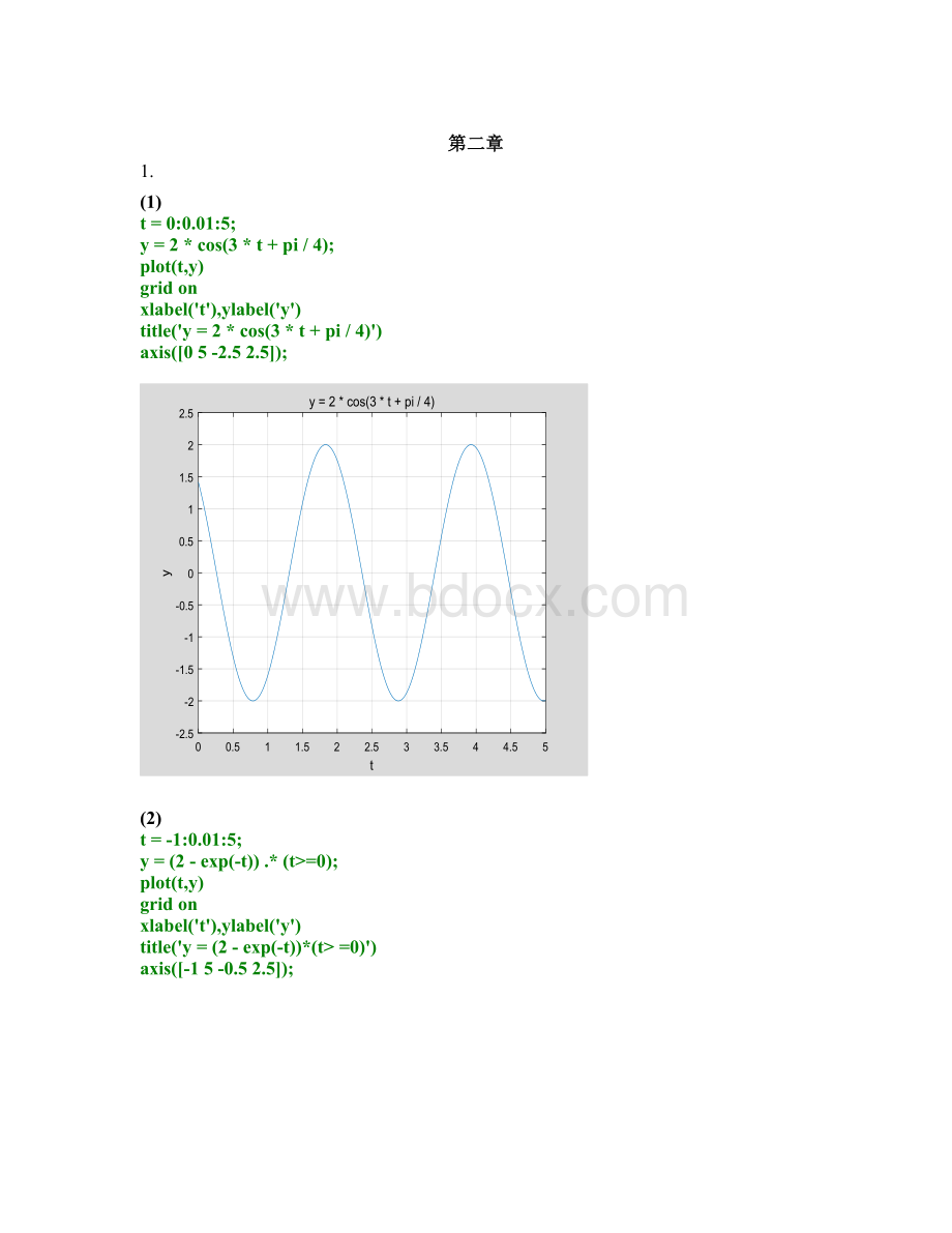
（1）

t=0:

0.01:

5;

y=2*cos（3*t+pi/4）;

plot（t,y）

gridon

xlabel（'t'）,ylabel（'y'）

title（'y=2*cos（3*t+pi/4）'）

axis（[05-2.52.5]）;

（2）

t=-1:

0.01:

5;

y=（2-exp（-t））.*（t>=0）;

plot（t,y）

gridon

xlabel（'t'）,ylabel（'y'）

title（'y=（2-exp（-t））*（t>=0）'）

axis（[-15-0.52.5]）;

（3）

t=-1:

0.01:

5;

y=t.*（（t>=0）-（（t-1）>=0））;

plot（t,y）

gridon

xlabel（'t'）,ylabel（'y'）

title（'y=t.*（（t>=0）-（（t-1）>=0））'）

axis（[-15-0.51.5]）;

（4）

t=-1:

0.01:

5;

y=（1+cos（pi*t））.*（（t>=0）-（（t-2）>=0））;

plot（t,y）

gridon

xlabel（'t'）,ylabel（'y'）

title（'y=（1+cos（pi*t））.*（（t>=0）-（（t-2）>=0））'）

axis（[-15-0.52.5]）;

2.

（1）

t=-4:

0.01:

10;

a=pi/4;

b=pi/2;

y=2+exp（（a*i）*t）+exp（（b*i）*t）;

subplot（2,2,1）;plot（t,real（y））;title（'实部'）;axis（[-41004.5]）;gridon;

subplot（2,2,2）;plot（t,imag（y））;title（'虚部'）;axis（[-410-34]）;gridon;

subplot（2,2,3）;plot（t,abs（y））;title（'模'）;axis（[-41004.5]）;gridon;

subplot（2,2,4）;plot（t,angle（y））;title（'相角'）;axis（[-410-1.51]）;gridon;

（2）

t=-4:

0.01:

10;

k=2;

b=pi/4;

y=k*exp（（t+b*i）*i）;

subplot（2,2,1）;plot（t,real（y））;title（'实部'）;axis（[-410-22]）;gridon;

subplot（2,2,2）;plot（t,imag（y））;title（'虚部'）;axis（[-410-34]）;gridon;

subplot（2,2,3）;plot（t,abs（y））;title（'模'）;axis（[-41002]）;gridon;

subplot（2,2,4）;plot（t,angle（y））;title（'相角'）;axis（[-410-44]）;gridon;

3.

P=2*pi;

t=0:

0.01:

5;

y=square（P*t,50）;

plot（t,y）

gridon;

axis（[06-21.5]）;

title（'幅度为1、周期为1,、占空比为0.5的周期矩形脉冲信号'）

第三章

1.

（1）

t=0:

0.01:

5;

y=exp（-t）.*sin（10*pi*t）+exp（-1/2*t）.*sin（9*pi*t）;

plot（t,y）

gridon;

title（'y=exp（-t）.*sin（10*pi*t）+exp（-1/2*t）.*sin（9*pi*t）'）

axis（[05-22]）

（2）

t=0:

0.01:

5;

y=sinc（t）.*cos（10*pi*t）;

plot（t,y）

gridon;

title（'y=sinc（t）.*cos（10*pi*t）'）

axis（[05-1.51.5]）

2.

定义一个函数

function[f]=fun（t）

f=（t+1）.*（heaviside（t+2）-heaviside（t+1））+heaviside（t+1）+heaviside（t）-heaviside（t-1）-heaviside（t-2）+（1-t）.*（heaviside（t-1）-heaviside（t-2））;

end

调用这个函数

t=-2:

0.01:

6;

f1=fun（t-1）;

f2=fun（2-t）;

f3=fun（2*t+1）;

f4=fun（4-t/2）;

f5=（fun（t）+fun（-t））.*（t>=0）;

subplot（231）;plot（t,f1）;title（'f（t-1）'）;axis（[-26-24]）;gridon

subplot（232）;plot（t,f2）;title（'f（2-t）'）;axis（[-26-24]）;gridon;

subplot（233）;plot（t,f3）;title（'f（2t+1）'）;axis（[-34-24]）;gridon;

subplot（234）;plot（t,f4）;title（'f（4-t/2）'）;axis（[-18-24]）;gridon;

subplot（235）;plot（t,f5）;title（'（f（t）+f（-t））u（t）'）;axis（[-35-24]）;gridon;

3．

t=0:

0.01:

3;

f=（heaviside（t）-heaviside（t-2））.*（1-t）;

f1=fliplr（f）;

fe=（f+f1）/2;

fo=（f-f1）/2;

subplot（1,2,1）;plot（t,fe）;title（'fe'）;gridon;

subplot（1,2,2）;plot（t,fo）;title（'fo'）;gridon;

第四章

1.

dt=0.001;t=-1:

dt:

3.5;

xt1=heaviside（t）-heaviside（t-2）;

xt2=heaviside（t）+heaviside（t-1）-heaviside（t-2）-heaviside（t-3）;

f=conv（xt1,xt2）*dt;

n=length（f）;

tt=（0:

n-1）*dt-2;

plot（tt,f）;gridon

第五章．

1.

（1）

dt=0.01;t=0:

dt:

4;

f=heaviside（t）;

sys=tf（[1],[1,4,3]）;

y=lsim（sys,f,t）;

plot（t,y）,gridon

xlabel（'t'）,ylabel（'y（t）'）

title（'零状态响应'）

（2）.

dt=0.01;t=0:

dt:

4;

f=exp（-t）.*heaviside（t）;

sys=tf（[1,3],[1,4,4]）;

y=lsim（sys,f,t）;

plot（t,y）,gridon

xlabel（'t'）,ylabel（'y（t）'）

title（'零状态响应'）

2.

（1）

t=0:

0.001:

4;

sys=tf（[1],[1,3,2]）;

h=impulse（sys,t）;

g=step（sys,t）;

subplot（1,2,1）;plot（t,h）;xlabel（'t'）,ylabel（'h（t）'）;title（'冲激响应'）;gridon

subplot（1,2,2）;plot（t,g）;xlabel（'t'）,ylabel（'g（t）'）;title（'阶跃响应'）;gridon

（2）

t=0:

0.001:

4;

sys=tf（[1,0],[1,2,2]）;

h=impulse（sys,t）;

g=step（sys,t）;

subplot（1,2,1）;plot（t,h）;xlabel（'t'）,ylabel（'h（t）'）;title（'冲激响应'）;gridon

subplot（1,2,2）;plot（t,g）;xlabel（'t'）,ylabel（'g（t）'）;title（'阶跃响应'）;gridon

第六章

1

T=2

所以函数傅里叶级数为

fx=12+4π2（cosπt+132cos3πt+152cos5πt+….）

注意：

以下代码需在MATLAB中运行才有多个图，在Word里运行只有一个图

t=-5:

0.001:

5;

omega=pi;

y=1/2+1/2*sawtooth（2*pi*1/2*（t+1）,0.5）;

plot（t,y）;axis（[-5,5,-0.3,1.1]）;gridon;xlabel（'t'）,ylabel（'y'）;title（'周期三角波的信号'）

n_max=[135913];

N=length（n_max）;

fork=1:

N

n=1:

2:

n_max（k）;

b=4./（pi*pi*n.*n）;

x=1/2+b*cos（omega*n'*t）;

figure;

plot（t,y）;

holdon;

plot（t,x）;

holdoff;

xlabel（'t'）,ylabel（'部分和的波形'）

axis（[-5,5,-0.3,1.1]）,gridon

title（['最大谐波数=',num2str（n_max（k））]）

end

2

r代表宽度，T代表周期

三角信号的傅里叶系数为A*Sa（2*pi/T）

n=-30:

30;T=2;w1=2*pi/T;

f=sinc（n*pi）;

subplot（311）;stem（n*w1,f）;axis（[-2020-12]）;gridon;title（'r=T=2'）

n=-30:

30;T=8;w1=2*pi/T;

f=sinc（n*pi）;

subplot（312）;stem（n*w1,f）;axis（[-2020-12]）;gridon;title（'r=T=8'）

n=-30:

30;T=16;w1=2*pi/T;

f=sinc（n*pi）;

subplot（313）;stem（n*w1,f）;axis（[-2020-12]）;gridon;title（'r=T=16'）

第七章

1.

（1）

f=sym（'sin（2*pi*（t-1））/（pi*（t-1））'）;

Fw=simplify（fourier（f））;

subplot（2,1,1）;ezplot（abs（Fw））;gridon;axis（[-44-12]）;title（'幅度谱'）

phase=atan（imag（Fw）/real（Fw））;

subplot（2,1,2）;ezplot（phase）;gridon;title（'相位谱'）

警告:

Supportofcharactervectorsthatarenotvalidvariablenamesordefineanumberwillberemovedinafuturerelease.Tocreatesymbolicexpressions,firstcreatesymbolicvariablesandthenuseoperationsonthem.

>Insym>convertExpression（line1559）

Insym>convertChar（line1464）

Insym>tomupad（line1216）

Insym（line179）

Fw

Fw=

-exp（-w*1i）*（heaviside（w-2*pi）-heaviside（w+2*pi））

（2）

fs=sinc（pi*t）;

f=sym（'fs^2'）;

Fw=simplify（fourier（f））

subplot（2,1,1）;ezplot（abs（Fw））;gridon;axis（[-44-12]）;title（'幅度谱'）

phase=atan（imag（Fw）/real（Fw））;

subplot（2,1,2）;ezplot（phase）;gridon;title（'相位谱'）

警告:

Supportofcharactervectorsthatarenotvalidvariablenamesordefineanumberwillberemovedinafuturerelease.Tocreatesymbolicexpressions,firstcreatesymbolicvariablesandthenuseoperationsonthem.

>Insym>convertExpression（line1559）

Insym>convertChar（line1464）

Insym>tomupad（line1216）

Insym（line179）

Fw=

-2*pi*dirac（2,w）

2.

（1）

symst;

Fw=sym（'10/（3+j*w）-4/（5+j*w）'）;

ft=simplify（ifourier（Fw,t））

ezplot（ft）,gridon

警告:

Supportofcharactervectorsthatarenotvalidvariablenamesordefineanumberwillberemovedinafuturerelease.Tocreatesymbolicexpressions,firstcreatesymbolicvariablesandthenuseoperationsonthem.

>Insym>convertExpression（line1559）

Insym>convertChar（line1464）

Insym>tomupad（line1216）

Insym（line179）

ft=

-（exp（-（t*5i）/j）*（sign（imag（1/j））-sign（t））*（5*exp（（t*2i）/j）-2）*1i）/j

（2）

symst

Fw=sym（'exp（-4*w^2）'）;

ft=simplify（ifourier（Fw,t））

ezplot（ft）,gridon

警告:

Supportofcharactervectorsthatarenotvalidvariablenamesordefineanumberwillberemovedinafuturerelease.Tocreatesymbolicexpressions,firstcreatesymbolicvariablesandthenuseoperationsonthem.

>Insym>convertExpression（line1559）

Insym>convertChar（line1464）

Insym>tomupad（line1216）

Insym（line179）

ft=

exp（-t^2/16）/（4*pi^（1/2））

3.

dt=0.01;t=-2:

dt:

2.5;

f=（heaviside（t+2）-heaviside（t+1））.*（t+2）+heaviside（t+1）-heaviside（t-1）+（heaviside（t-1）-heaviside（t-2））.*（2-t）;

N=100;

k=-N:

N;

W=pi*k/（N*dt）;

Fw=f*exp（-i*t'*W）*dt;

plot（W,abs（Fw））;gridon;axis（[-5*pi5*pi-0.14]）;title（'频谱图'）

4.

由题可知，两个门函数完全相同，才能得到三角形脉冲

首先将门函数进行时域卷积运算，再将卷积后的结果做傅里叶变换，源程序如下：

dt=0.01;t=-2:

dt:

2.5;

f1=heaviside（t+0.5）-heaviside（t-0.5）;%定义一个门函数

f=conv（f1,f1）*dt;%卷积运算

ft=sym（'f'）;

Fw=fourier（ft）%对卷积运算所得结果进行傅里叶变换

Fw=

pi*dirac（1,w）*2i

再求出一个门函数进行傅里叶变换，再与自身相乘，如果下面所得结果与上述Fw相同，说明验证了傅里叶变换的时域卷积定理，源程序如下：

dt=0.01;t=-2:

dt:

2.5;

f1=heaviside（t+0.5）-heaviside（t-0.5）;

ft=sym（'f1'）;

Fw1=fourier（ft）;

Fw=Fw1'*Fw1

Fw=

4*pi^2*dirac（1,w）^2

第八章

1.

由图可知，该电路频率响应为H（w）=jw/（0.2（jw）^3+0.2（jw）^2+jw）

w=-6*pi:

0.01:

6*pi;

b=[100];

a=[22100];

H=freqs（b,a,w）;

subplot（2,1,1）;plot（w,abs（H））;gridon;xlabel（'\omega（rad/s）'）,ylabel（'|H（\omega）|'）;title（'电路系统的幅频特性'）

subplot（2,1,2）;plot（w,angle（H））;xlabel（'\omega（rad/s）'）,ylabel（'\phi（\omega）'）;gridon;title（'电路系统的相频特性'）

2.

（1）

频率响应为H（w）=jw/（jw+3/2）

t=0:

0.01:

20;

H=（w*j）/（w*j+3/2）;

f=cos（2*t）;

y=abs（H）*cos（2*t+angle（H））;

subplot（211）;plot（t,f）;gridon;title（'激励信号的波形'）

subplot（212）;plot（t,y）;gridon;title（'稳态响应的波形'）

（2）

t=0:

0.01:

20;

w1=2;w2=5;

H1=（-1i*w1+2）./（（1i*w1）^2+2*1i*w1+3）;

H2=（-1i*w2+2）./（（1i*w2）^2+2*1i*w2+3）;

f=3+cos（2*t）+cos（5*t）;

y=3+abs（H1）*cos（w1*t+angle（H1））+abs（H2）*cos（w2*t+angle（H2））;

plot（t,y）;gridon;title（'稳态响应的波形'）

第九章

1.

Ts=0.00025;

dt=0.0001;

t1=-0.1:

dt:

0.1;

ft=sin（200*pi*t1）;

subplot（221）;plot（t1,ft）;gridon;axis（[-0.010.01-1.11.1]）;title（'f1的信号'）

N=100;

k=-N:

N;

W=pi*k/（N*dt）;

Fw=ft*exp（-i*t1'*W）*dt;

subplot（222）;plot（W,abs（Fw））;gridon;axis（[-50005000-0.10.2]）;title（'f1信号的频谱'）

t2=-0.1:

Ts:

0.1;

fst=sin（200*pi*t2）;

subplot（223）;plot（t1,ft,':

'）;holdon;stem（t2,fst）;gridon;axis（[-0.010.01-1.11.1]）;title（'抽样后的信号'）;holdoff

Fsw=fst*exp（-i*t2'*W）*Ts;

subplot（224）;plot（W,abs（Fsw））;gridon;axis（[-50005000-0.10.2]）;title（'抽样信号的频谱'）

2.

symst;

Sa（t）=sin（t）./t;

subplot（211）;ezplot（Sa（t））;gridon;title（'Sa（t）函数的波形'）

Fw=simplify（fourier（Sa（t）））;

subplot（212）;ezplot（abs（Sa（t）））;gridon;xlabel（'\omega'）,ylabel（'H（jw）'）;title（'Sa（t）的频谱'）

由图可知，Sa（t）的频谱大部分集中在[0,6]之间，所以可设其截至频率Wm=6,因而Ts=pi/6;

采用截至频率Wc=1.2Wm的低通滤波器对抽样信号滤波后重建信号法f（t）,并计算重建信号与原Sa（t）信号的绝对误差

Wm=6;

Wc=1.2*Wm;

Ts=0.4;

n=-100:

100;

nTs=n*Ts;

fs=sinc（nTs/pi）;

t=-6:

0.1:

6;

ft=Ts*Wc/pi*fs*sinc（（Wc/pi）*（ones（length（nTs）,1）*t）-nTs'*ones（1,length（t）））;

t1=-6:

0.1:

6;

f1=sinc（t1/pi）;

subplot（311）;plot（t1,f1,':

'）,holdon;stem（nTs,fs）;axis（[-66-11]）;xlabel（'nTs'