SPSS使用详解.docx
《SPSS使用详解.docx》由会员分享,可在线阅读,更多相关《SPSS使用详解.docx(18页珍藏版)》请在冰豆网上搜索。
SPSS使用详解
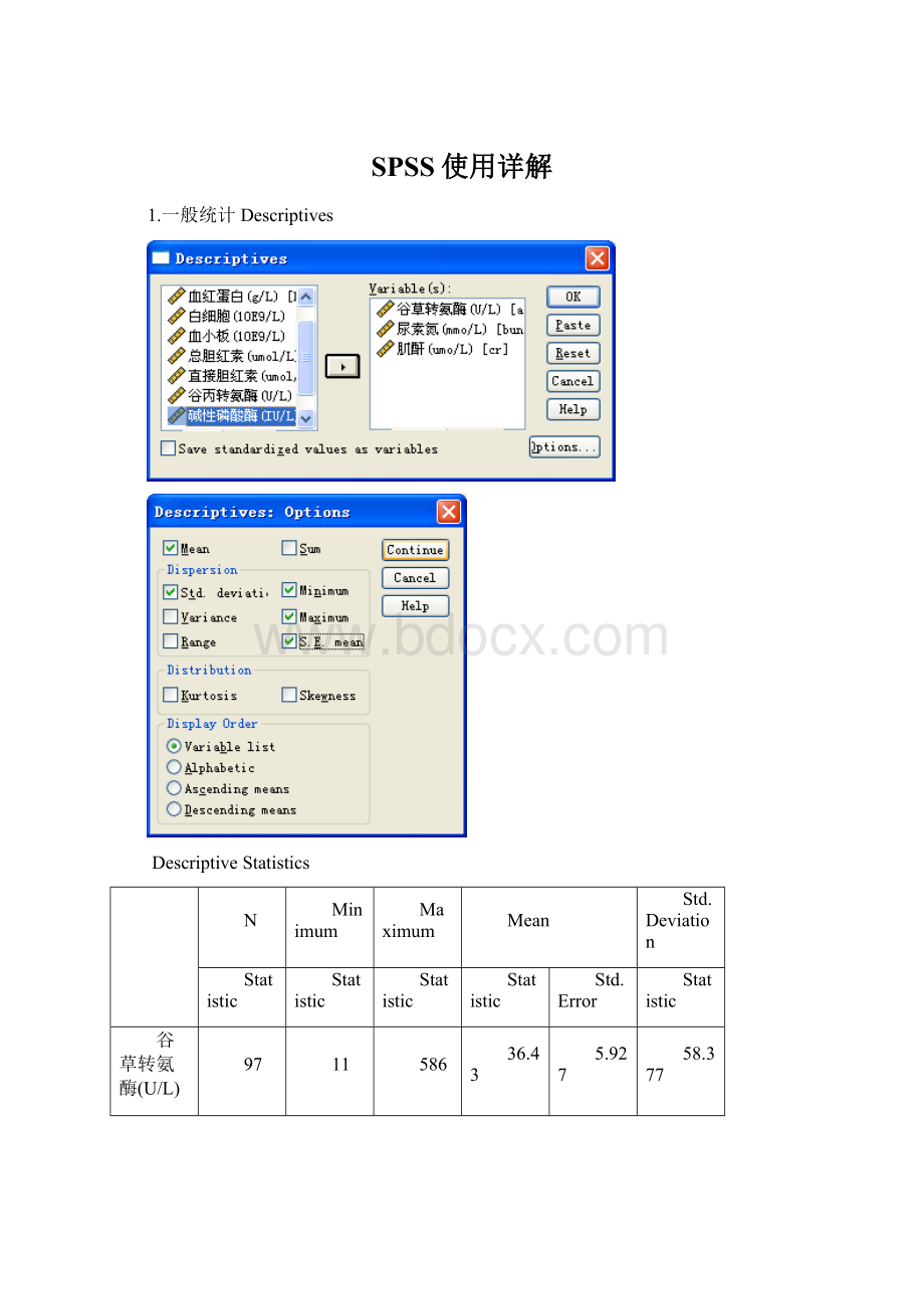
1.一般统计Descriptives
DescriptiveStatistics
N
Minimum
Maximum
Mean
Std.Deviation
Statistic
Statistic
Statistic
Statistic
Std.Error
Statistic
谷草转氨酶(U/L)
97
11
586
36.43
5.927
58.377
尿素氮(mmo/L)
97
2.0
18.4
5.096
.2558
2.5189
肌酐(umo/L)
97
28
190
82.06
2.275
22.407
ValidN(listwise)
97
2.均数比较(comparemeans)
1.独立样本t检验,Independent-sampleTTest
比较2个样本之间的均数是否有显著差异,亦称two-sampleTTest.
工厂的两个化验室,每天对所配的水样,分别测定其含氯量(ppm),下面是7天的记录,问:
两化验室测定结果之间有无显著差异?
(α=0.01)。
日期
1
2
3
4
5
6
7
化验室A
1.15
1.86
0.75
1.82
1.14
1.65
1.90
化验室B
1.00
1.90
0.90
1.80
1.20
1.70
1.95
数据定义(格式)
Group
Cl
1
1.15
1
1.86
1
0.75
1
1.82
1
1.14
1
1.65
1
1.9
2
1
2
1.9
2
0.9
2
1.8
2
1.2
2
1.7
2
1.95
数据分析
IndependentSamplesTest
Levene'sTestforEqualityofVariances方差齐性检验
t-testforEqualityofMeans
F
Sig.
t
df
Sig.(2-tailed)
MeanDifference
Std.ErrorDifference
99%ConfidenceIntervaloftheDifference
Lower
Upper
Lower
Upper
Lower
Upper
Lower
Upper
Lower
Cl
Equalvariancesassumed
.004
.952
-.107
12
.916
-.02571
.23973
-.75797
.70654
Equalvariancesnotassumed
-.107
11.998
.916
-.02571
.23973
-.75799
.70656
2.配对样本T检验pairedsampleTtest
与onesampleTtest类似
3.单向方差分析OnewayANOVA
用于完全随机设计资料中的多个样本均数比较和样本均数之间的多种比较,亦可进行多个处理与一个对照组的比较。
例:
黑龙江某地淋溶土上玉米氮肥品种肥效试验,每亩施N6斤,小区面积54m2,随机区组设计,重复四次,玉米产量见下表:
重复
产量(公斤/亩)
CK
碳铵
硫铵
硝铵
氰铵
尿素
氯铵
氨水
1
126.8
233.8
261.0
277.2
196.4
272.5
264.6
253.4
2
148.7
231.1
263.3
268.7
208.9
246.1
252.9
274.1
3
121.9
226.0
248.4
291.7
203.1
269.4
267.5
246.3
4
83.1
221.3
259.2
255.4
141.6
232.5
150.3
251.9
解题:
1.建立数据矩阵,按照SPSS格式重新编排数据
处理
产量
1
126.8
1
148.7
1
121.9
1
83.1
2
233.8
2
231.1
2
226
2
221.3
3
261
3
263.3
3
248.4
3
259.2
4
277.2
4
268.7
4
291.7
4
255.4
5
196.4
5
208.9
5
203.1
5
141.6
6
272.5
6
246.1
6
269.4
6
232.5
7
264.6
7
252.9
7
267.5
7
150.3
8
253.4
8
274.1
8
246.3
8
251.9
2.在SPSS内新建立一个数据,定义变量和输入数据
变量名:
Name,随机取,
标签:
label,
变量值:
Value
其他选项不用设置,以上3个也可以不设置,采用默认,
好处:
定义后会给后面的数据分析提供便利,利于分析。
3.调用模块进行数据分析,Means:
)OnewayANOVA
设置比较方法:
PostHoc
结果显示
ANOVA
产量
平方和
df
均方
F
显著性
组间
71135.295
7
10162.185
14.342
.000
组内
17005.517
24
708.563
总数
88140.812
31
多重比较
产量LSD
(I)氮肥种类
(J)氮肥种类
均值差(I-J)
标准误
显著性
95%置信区间
下限
上限
CK
碳铵
-107.92500*
18.82237
.000
-146.7725
-69.0775
硫铵
-137.85000*
18.82237
.000
-176.6975
-99.0025
硝铵
-153.12500*
18.82237
.000
-191.9725
-114.2775
氰铵
-67.37500*
18.82237
.002
-106.2225
-28.5275
尿素
-135.00000*
18.82237
.000
-173.8475
-96.1525
氯铵
-113.70000*
18.82237
.000
-152.5475
-74.8525
氨水
-136.30000*
18.82237
.000
-175.1475
-97.4525
*.均值差的显著性水平为0.05。
分析:
1.CK与其他各种氮肥均有显著性差异。
。
。
。
。
4.GLM(generallinermodel)
1.单变量方差分析(Univariate)
它包含了一般方差分析的方法,如one-wayANOVA
既可分析各个因素对一个反应变量的主效应,亦可分析各因子之间的交互效应。
单因素随机区组设计
例:
黑龙江某地淋溶土上玉米氮肥品种肥效试验,每亩施N6斤,小区面积54m2,随机区组设计,重复四次,玉米产量见下表:
重复
产量(公斤/亩)
CK
碳铵
硫铵
硝铵
氰铵
尿素
氯铵
氨水
1
126.8
233.8
261.0
277.2
196.4
272.5
264.6
253.4
2
148.7
231.1
263.3
268.7
208.9
246.1
252.9
274.1
3
121.9
226.0
248.4
291.7
203.1
269.4
267.5
246.3
4
83.1
221.3
259.2
255.4
141.6
232.5
150.3
251.9
解题:
同样按照上面的方法建立数据文件,选择GLM----Univariate
TestsofBetween-SubjectsEffects
DependentVariable:
产量
Source
TypeIIISumofSquares
df
MeanSquare
F
Sig.
CorrectedModel
71135.295(a)
7
10162.185
14.342
.000
Intercept
1642170.338
1
1642170.338
2317.606
.000
N_type
71135.295
7
10162.185
14.342
.000
Error
17005.518
24
708.563
Total
1730311.150
32
CorrectedTotal
88140.812
31
aRSquared=.807(AdjustedRSquared=.751)
多重比较结果同上
多因素随机区组设计
假设某试验为二种冬小麦品种(A1、A2),二种密度(B1、B2),三种氮肥用量(C1、C2、C3)的三因素随机区组设计,试验小区面积为0.05亩,重复三次,产量结果见下表。
重复
处理
1
2
3
A1B1C1
5
6
7
A1B1C2
15
16
17
A1B1C3
21
22
23
A1B2C1
10
12
22
A1B2C2
20
22
21
A1B2C3
22
23
24
A2B1C1
25
26
27
A2B1C2
30
33
36
A2B1C3
30
32
34
A2B2C1
19
22
22
A2B2C2
25
27
26
A2B2C3
23
24
22
解题:
1.
冬小麦品种
密度
氮肥用量
产量
1
1
1
5
1
1
1
6
1
1
1
7
1
1
2
15
1
1
2
16
1
1
2
17
1
1
3
21
1
1
3
22
1
1
3
23
1
2
1
10
1
2
1
12
1
2
1
22
1
2
2
20
1
2
2
22
1
2
2
21
1
2
3
22
1
2
3
23
1
2
3
24
2
1
1
25
2
1
1
26
2
1
1
27
2
1
2
30
2
1
2
33
2
1
2
36
2
1
3
30
2
1
3
32
2
1
3
34
2
2
1
19
2
2
1
22
2
2
1
22
2
2
2
25
2
2
2
27
2
2
2
26
2
2
3
23
2
2
3
24
2
2
3
22
2.选择GLM模块的Univariate程序,确定变量
3.选择模型Model,可默认,不进行设置
4.选择比较方法把需要比较的因素选入右侧框内,然后选择比较方法Duncan(SSR)
Warnings
Posthoctestsarenotperformedfor密度becausetherearefewerthanthreegroups.
Posthoctestsarenotperformedfor小麦品种becausetherearefewerthanthreegroups.
在spss中Posthoctests适用于作多组(大于等于3)的多重比较的,如果总共只有2个组就没有必要做多重比较了,方差分析给出的结果已经是这两组的比较结果了。
TestsofBetween-SubjectsEffects
DependentVariable:
产量
Source
TypeIIISumofSquares
df
MeanSquare
F
Sig.
CorrectedModel
1808.306(a)
11
164.391
30.194
.000
Intercept
17380.028
1
17380.028
3192.250
.000
fertiliser
466.056
2
233.028
42.801
.000
density
10.028
1
10.028
1.842
.187
wheat
850.694
1
850.694
156.250
.000
fertiliser*density
51.056
2
25.528
4.689
.019
fertiliser*wheat
107.389
2
53.694
9.862
.001
density*wheat
318.028
1
318.028
58.413
.000
fertiliser*density*wheat
5.056
2
2.528
.464
.634
Error
130.667
24
5.444
Total
19319.000
36
CorrectedTotal
1938.972
35
5.相关和回归分析
双变量相关分析(Biovariate)
Correlations
年龄(岁)
限制性端粒片断长度(bp)
年龄(岁)
PearsonCorrelation
1
-.732(**)
Sig.(2-tailed)
.000
N
123
123
限制性端粒片断长度(bp)
PearsonCorrelation
-.732(**)
1
Sig.(2-tailed)
.000
N
123
123
**Correlationissignificantatthe0.01level(2-tailed).
偏相关分析(partial)
线性回归linearregression
某克山病区10名健康儿童头发与血液中的硒含量测定结果如下,试作相关分析,若发硒与血硒含量之间存在直线关系,拟作自发硒推算血硒(y)的回归分析。
发硒(x)
74
66
88
69
91
73
66
96
58
73
血硒(y)
13
10
13
11
16
9
7
14
5
10
ANOVA(b)
Model
SumofSquares
df
MeanSquare
F
Sig.
1
Regression
75.649
1
75.649
25.268
.001(a)
Residual
23.951
8
2.994
Total
99.600
9
aPredictors:
(Constant),发硒
bDependentVariable:
血硒
Coefficients(a)
Model
UnstandardizedCoefficients
StandardizedCoefficients
t
Sig.
B
Std.Error
Beta
B
Std.Error
1
(Constant)
-6.980
3.579
-1.950
.087
发硒
.236
.047
.872
5.027
.001
aDependentVariable:
血硒
 升级会员
升级会员 