《信号与系统》实验三.docx
《《信号与系统》实验三.docx》由会员分享,可在线阅读,更多相关《《信号与系统》实验三.docx(18页珍藏版)》请在冰豆网上搜索。
《信号与系统》实验三
信息科学与工程学院《信号与系统》实验报告三
专业班级电信(DB)1002班姓名周攀学号201012135055
实验时间2012年4月27日指导教师陈华丽成绩
实验
名称
连续信号的频域分析
实验
目的
1.掌握周期信号的频谱——Fourier级数的分析方法及其物理意义。
2.深入理解信号频谱的概念,掌握典型信号的频谱以及Fourier变换的主要性质。
实验
内容
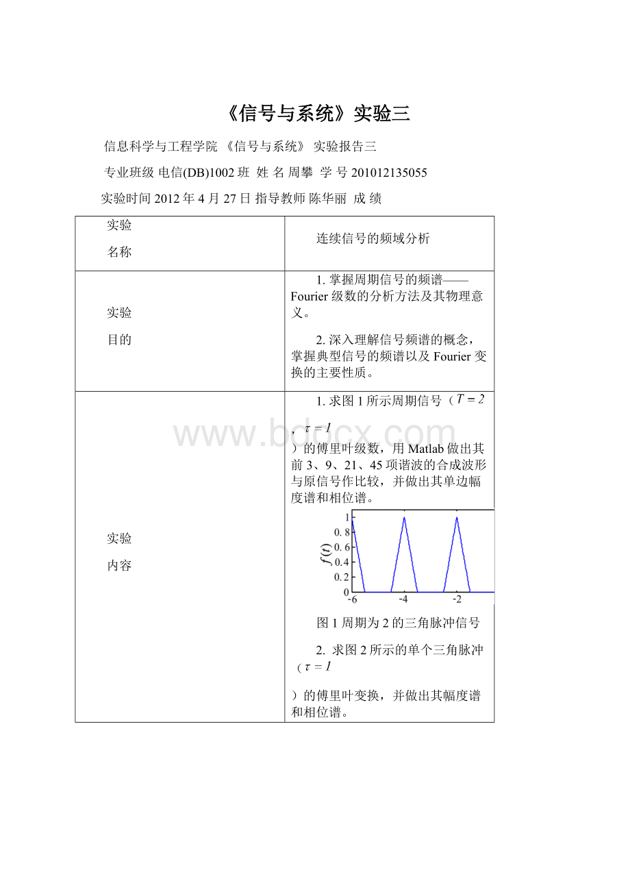
1.求图1所示周期信号(
,
)的傅里叶级数,用Matlab做出其前3、9、21、45项谐波的合成波形与原信号作比较,并做出其单边幅度谱和相位谱。
图1周期为2的三角脉冲信号
2.求图2所示的单个三角脉冲(
)的傅里叶变换,并做出其幅度谱和相位谱。
图2单个三角脉冲
3.求不同占空比下周期矩形脉冲的幅度谱和相位谱,例如
、
。
4.验证傅里叶变换的性质:
(选作)
a)时移性质:
选取
和
,幅频曲线相同,只有相位不同。
b)频移性质:
选取
和
或
。
c)对称性质:
选取
和
。
d)尺度变换性:
选取
和
。
实验记录及个人小结(包括:
实验源程序、注释、结果分析与讨论等)
1.t=-6:
0.01:
6;functiony=fourierseries(m,t)
d=-6:
2:
6;y=1/4;
fxx=pulstran(t,d,'tripuls');forn=1:
m
f1=fourierseries(3,t);y=y+4/(n*n*pi*pi)*(1-cos(n*pi/2)).*cos(n*pi.*t);
f2=fourierseries(9,t);end
f3=fourierseries(21,t);
f4=fourierseries(45,t);
subplot(2,2,1)
plot(t,fxx,'r',t,f1,'b');
gridon
axis([-66-0.11.1])
title('N=3')
subplot(2,2,2)
plot(t,fxx,'r',t,f2,'b');
gridon
axis([-66-0.11.1])
title('N=9')
subplot(2,2,3)
plot(t,fxx,'r',t,f3,'b');
gridon
axis([-66-0.11.1])
title('N=21')
subplot(2,2,4)
plot(t,fxx,'r',t,f4,'b');
gridon
axis([-66-0.11.1])
title('N=45')
n=1:
10;
a=zeros(size(n));
a
(1)=0.5;
forii=2:
10
a(ii)=abs(4/((ii-1)*(ii-1)*pi*pi)*(1-cos((ii-1)*pi/2)))
end
n=0:
pi:
9*pi
stem(n,a,'fill','linewidth',2);
axis([0,9*pi,0,0.5])
gridon
title('\it单边幅度谱')
xlabel('\fontsize{14}\bfΩ=nΩo\rightarrow')
ylabel('\fontsize{14}\bfAn\rightarrow')
n=1:
10;
a=zeros(size(n));
fori=1:
10
a(i)=angle(4/(i*i*pi*pi)*(1-cos(i*pi/2)))
end
n=0:
pi:
9*pi
stem(n,a,'fill','linewidth',2);
axis([0,9*pi,-0.2,0.2])
gridon
title('\it单边相位谱')
xlabel('\fontsize{14}\bfΩ=nΩo\rightarrow')
ylabel('\fontsize{14}\bfΨn\rightarrow')\bfΨn\rightarrow')
2.t=-6:
0.001:
6;
d=0
f=pulstran(t,d,'tripuls')
T=0.01;dw=0.1;
w=-10*pi:
dw:
10*pi;
F=f*exp(-j*t'*w)*T;
F1=abs(F);
phaF=angle(F);
subplot(2,1,1)
plot(w,F1);
axis([-10*pi,10*pi,0,5])
gridon
title('\it幅度谱')
xlabel('\fontsize{14}\bfw\rightarrow')
ylabel('\fontsize{14}\bf|Fn|\rightarrow')
subplot(2,1,2)
plot(w,phaF);
title('\it相位谱')
xlabel('\fontsize{14}\bfw\rightarrow')
ylabel('\fontsize{14}\bfΨn\rightarrow')
gridon
3.n=-20:
20;
F=zeros(size(n));
forii=-20:
20
F(ii+21)=sin(ii*pi/4)/(ii*pi+eps);
end
F(21)=1/4;
F1=abs(F);
phaF=angle(F);
subplot(2,1,1)
stem(n,F1,'fill')
title('\it周期矩形脉冲的幅度谱(τ/T=1/4)')
xlabel('\fontsize{14}\bfn\rightarrow')
ylabel('\fontsize{14}\bf|Fn|\rightarrow')
subplot(2,1,2)
stem(n,phaF,'fill')
title('\it周期矩形脉冲的相位谱(τ/T=1/4)')
xlabel('\fontsize{14}\bfn\rightarrow')
ylabel('\fontsize{14}\bfΨn\rightarrow')
n=-20:
20;
F=zeros(size(n));
forii=-20:
20
F(ii+21)=sin(ii*pi/8)/(ii*pi+eps);
end
F(21)=1/8;
F1=abs(F);
phaF=angle(F);
subplot(2,1,1)
stem(n,F1,'fill')
title('\it周期矩形脉冲的幅度谱(τ/T=1/8)')
xlabel('\fontsize{14}\bfn\rightarrow')
ylabel('\fontsize{14}\bf|Fn|\rightarrow')
subplot(2,1,2)
stem(n,phaF,'fill')
title('\it周期矩形脉冲的相位谱(τ/T=1/8)')
xlabel('\fontsize{14}\bfn\rightarrow')
ylabel('\fontsize{14}\bfΨn\rightarrow')
4.(a).
T=0.01;
t=-10:
0.01:
10;
dw=0.1;
w=-4*pi:
dw:
4*pi;
F1=rectpuls(t)*exp(-j*t'*w)*T;
F2=rectpuls(t-6)*exp(-j*t'*w)*T;
a1=abs(F1);
phaF1=angle(F1);
a2=abs(F2);
phaF2=angle(F2);
subplot(2,2,1)
plot(w,a1);
title('\it幅度谱')
xlabel('\fontsize{14}\bfw\rightarrow')
ylabel('\fontsize{14}\bf|Fn|\rightarrow')
subplot(2,2,2)
plot(w,phaF1);
title('\it相位谱')
xlabel('\fontsize{14}\bfw\rightarrow')
ylabel('\fontsize{14}\bfΨn\rightarrow')
subplot(2,2,3)
plot(w,a2);
title('\it幅度谱')
xlabel('\fontsize{14}\bfw\rightarrow')
ylabel('\fontsize{14}\bf|Fn|\rightarrow')
subplot(2,2,4)
plot(w,phaF2);
title('\it相位谱')
xlabel('\fontsize{14}\bfw\rightarrow')
ylabel('\fontsize{14}\bfΨn\rightarrow')
(b).
T=0.01;
t=-10:
0.01:
10;
dw=0.1;
w=-4*pi:
dw:
4*pi;
f1=u(t).*sin(3*t);
F1=u(t)*exp(-j*t'*w)*T;
F2=f1*exp(-j*t'*w)*T;
a1=abs(F1);
phaF1=angle(F1);
a2=abs(F2);
phaF2=angle(F2);
subplot(2,2,1)
plot(w,a1);
title('\it幅度谱')
xlabel('\fontsize{14}\bfw\rightarrow')
ylabel('\fontsize{14}\bf|F1n|\rightarrow')
subplot(2,2,2)
plot(w,phaF1);
title('\it相位谱')
xlabel('\fontsize{14}\bfw\rightarrow')
ylabel('\fontsize{14}\bfΨ1n\rightarrow')
subplot(2,2,3)
plot(w,a2);
title('\it幅度谱')
xlabel('\fontsize{14}\bfw\rightarrow')
ylabel('\fontsize{14}\bf|F2n|\rightarrow')
subplot(2,2,4)
plot(w,phaF2);
title('\it相位谱')
xlabel('\fontsize{14}\bfw\rightarrow')
ylabel('\fontsize{14}\bfΨ2n\rightarrow')
(c).
T=0.01;
t=-10:
0.01:
10;
dw=0.1;
w=-4*pi:
dw:
4*pi;
y=sinc(2*t/pi);
F1=y*exp(-j*t'*w)*T;
F2=g(t)*exp(-j*t'*w)*T;
a1=abs(F1);
phaF1=angle(F1);
a2=abs(F2);
phaF2=angle(F2);
subplot(2,2,1)
plot(w,a1);
title('\it幅度谱')
xlabel('\fontsize{14}\bfw\rightarrow')
ylabel('\fontsize{14}\bf|F1n|\rightarrow')
subplot(2,2,2)
plot(w,phaF1);
title('\it相位谱')
xlabel('\fontsize{14}\bfw\rightarrow')
ylabel('\fontsize{14}\bfΨ1n\rightarrow')
subplot(2,2,3)
plot(w,a2);
title('\it幅度谱')
xlabel('\fontsize{14}\bfw\rightarrow')
ylabel('\fontsize{14}\bf|F2n|\rightarrow')
subplot(2,2,4)
plot(w,phaF2);
title('\it相位谱')
xlabel('\fontsize{14}\bfw\rightarrow')
ylabel('\fontsize{14}\bfΨ2n\rightarrow')
(d).
T=0.01;
t=-10:
0.01:
10;
dw=0.1;
w=-4*pi:
dw:
4*pi;
F1=rectpuls(t)*exp(-j*t'*w)*T;
F2=rectpuls(2*t)*exp(-j*t'*w)*T;
a1=abs(F1);
phaF1=angle(F1);
a2=abs(F2);
phaF2=angle(F2);
subplot(2,2,1)
plot(w,a1);
title('\it幅度谱')
xlabel('\fontsize{14}\bfw\rightarrow')
ylabel('\fontsize{14}\bf|F1n|\rightarrow')
subplot(2,2,2)
plot(w,phaF1);
title('\it相位谱')
xlabel('\fontsize{14}\bfw\rightarrow')
ylabel('\fontsize{14}\bfΨ1n\rightarrow')
subplot(2,2,3)
plot(w,a2);
title('\it幅度谱')
xlabel('\fontsize{14}\bfw\rightarrow')
ylabel('\fontsize{14}\bf|F2n|\rightarrow')
subplot(2,2,4)
plot(w,phaF2);
title('\it相位谱')
xlabel('\fontsize{14}\bfw\rightarrow')
ylabel('\fontsize{14}\bfΨ2n\rightarrow')
 升级会员
升级会员 