最新R语言因子实验设计和解释案例分析报告 附代码数据.docx

最新R语言因子实验设计和解释案例分析报告 附代码数据.docx

《最新R语言因子实验设计和解释案例分析报告 附代码数据.docx》由会员分享，可在线阅读，更多相关《最新R语言因子实验设计和解释案例分析报告 附代码数据.docx（22页珍藏版）》请在冰豆网上搜索。

最新R语言因子实验设计和解释案例分析报告附代码数据

R语言因子实验设计和解释案例分析报告

·示例1：

两组比较

·示例2：

多个组

实例3：

两个条件，两个基因型，一个交互项

o野生型治疗效果（主效应）。

o突变体治疗的效果

o没有治疗的突变型和野生型之间有什么区别？

o通过治疗，突变型和野生型有什么区别？

o基因型的不同反应（相互作用项）

实例4：

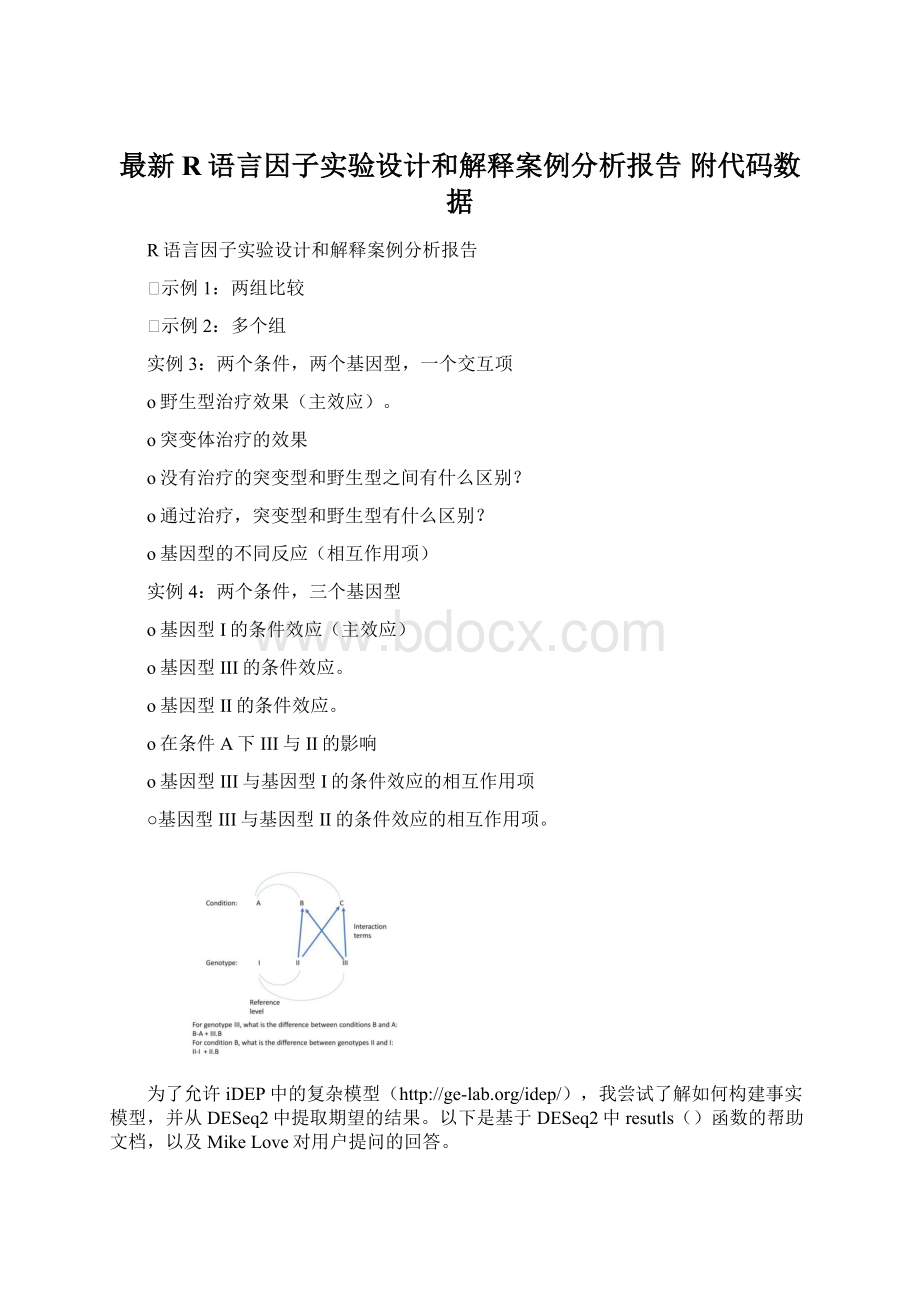
两个条件，三个基因型

o基因型I的条件效应（主效应）

o基因型III的条件效应。

o基因型II的条件效应。

o在条件A下III与II的影响

o基因型III与基因型I的条件效应的相互作用项

○基因型III与基因型II的条件效应的相互作用项。

为了允许iDEP中的复杂模型（http:

//ge-lab.org/idep/），我尝试了解如何构建事实模型，并从DESeq2中提取期望的结果。

以下是基于DESeq2中resutls（）函数的帮助文档，以及MikeLove对用户提问的回答。

我想要做的一个重点是，当研究设计涉及多个因素时（参见上面关于基因型+治疗实例的图），结果的解释是棘手的。

与R中的回归分析类似，分类因素的参考水平构成了我们的分歧的基础。

然而，默认情况下，它们是按字母顺序确定的。

选择每个因素的参考水平是至关重要的。

否则你的系数可能会有所不同，这取决于你如何进入DESeq2的实验设计。

这可以通过R中的relevel（）函数完成。

参考级别是构成有意义比较基础的因素的基线级别。

在野生型与突变型实验中，“野生型”是参考水平。

在治疗与未治疗，参考水平显然是未经处理的。

例3中的更多细节。

例1：

两组比较

首先制作一些示例数据。

library（DESeq2）

dds<-makeExampleDESeqDataSet（n=10000,m=6）

assay（dds）[1:

10,]

##sample1sample2sample3sample4sample5sample6

##gene164111213

##gene291223131428

##gene35812117317811897

##gene4040383

##gene527369812

##gene648835382113

##gene7365061524422

##gene86816141819

##gene9214266419198157166

##gene1020121612162

这是一个非常简单的实验设计，有两个条件。

colData（dds）

##DataFramewith6rowsand1column

##condition

##

##sample1A

##sample2A

##sample3A

##sample4B

##sample5B

##sample6B

dds<-DESeq（dds）

resultsNames（dds）

##[1]"Intercept""condition_B_vs_A"

这显示了可用的结果。

请注意，默认情况下，R会根据字母顺序为因素选择一个参考级别。

这里A是参考水平。

折叠变化定义为B与A比较。

要更改参考级别，请尝试使用“同一个”（）函数。

res<-results（dds,contrast=c（"condition","B","A"））

res<-res[order（res$padj）,]

library（knitr）

kable（res[1:

5,-（3:

4）]）

baseMean

log2FoldChange

pvalue

padj

gene9056

360.168909

-2.045379

0.0000000

0.0001366

gene3087

43.897516

-2.203303

0.0000173

0.0858143

gene3763

72.409877

-1.834787

0.0000434

0.1434712

gene2054

322.494963

1.537408

0.0000681

0.1689463

gene4617

6.227415

6.125238

0.0002019

0.4008408

如果我们想用B作为控制，并用B作为基线定义倍数变化。

那我们可以这样做：

res<-results（dds,contrast=c（"condition","A","B"））

ix=which.min（res$padj）

res<-res[order（res$padj）,]

kable（res[1:

5,-（3:

4）]）

baseMean

log2FoldChange

pvalue

padj

gene9056

360.168909

2.045379

0.0000000

0.0001366

gene3087

43.897516

2.203303

0.0000173

0.0858143

gene3763

72.409877

1.834787

0.0000434

0.1434712

gene2054

322.494963

-1.537408

0.0000681

0.1689463

gene4617

6.227415

-6.125238

0.0002019

0.4008408

正如你所看到的，折叠的方向是完全相反的。

这里我们展示最重要的基因。

barplot（assay（dds）[ix,],las=2,main=rownames（dds）[ix]）

示例2：

多个组

假设我们有三个组A，B和C.

dds<-makeExampleDESeqDataSet（n=100,m=6）

dds$condition<-factor（c（"A","A","B","B","C","C"））

dds<-DESeq（dds）

res=results（dds,contrast=c（"condition","C","A"））

res<-res[order（res$padj）,]

kable（res[1:

5,-（3:

4）]）

baseMean

log2FoldChange

pvalue

padj

gene2

3.634986

-5.101773

0.0348679

0.5515088

gene20

4.678176

-4.490982

0.0445664

0.5515088

gene34

56.068672

-1.462155

0.0167820

0.5515088

gene35

537.847175

-1.177240

0.0087913

0.5515088

gene41

93.967810

1.064734

0.0412034

0.5515088

Example3:

twoconditions,twogenotypes,withaninteractionterm

Herewehavetwogenotypes,wild-type（WT）,andmutant（MU）.Twoconditions,control（Ctrl）andtreated（Trt）.Weareinterestedintheresponsesofbothwild-typeandmutanttotreatment.Wearealsointerestedinthedifferencesinresponsebetweengenotypes,whichiscapturedbytheinteractionterminlinearmodels.

First,weconstructexampledata.Notethatwechangedsamplenamesfrom“sample1”to“Wt_Ctrl_1”,accordingtothetwofactors.

dds<-makeExampleDESeqDataSet（n=10000,m=12）

dds$condition<-factor（c（rep（"Ctrl",6）,rep（"Trt",6）））

dds$genotype<-factor（rep（rep（c（"WT","MU"）,each=3）,2））

colnames（dds）<-paste（as.character（dds$genotype）,as.character（dds$condition）,rownames（colData（dds））,sep="_"）

colnames（dds）=gsub（"sample","",colnames（dds））

kable（assay（dds）[1:

5,]）

WT_Ctrl_1

WT_Ctrl_2

WT_Ctrl_3

MU_Ctrl_4

MU_Ctrl_5

MU_Ctrl_6

WT_Trt_7

WT_Trt_8

WT_Trt_9

MU_Trt_10

MU_Trt_11

MU_Trt_12

gene1

81

47

135

72

81

80

76

57

52

49

64

57

gene2

70

77

94

54

54

36

51

66

57

51

47

67

gene3

16

37

8

28

4

36

14

10

7

11

40

15

gene4

2

5

1

3

9

2

1

5

0

0

14

8

gene5

0

0

1

0

5

0

0

0

0

0

0

0

kable（colData（dds））

condition

genotype

WT_Ctrl_1

Ctrl

WT

WT_Ctrl_2

Ctrl

WT

WT_Ctrl_3

Ctrl

WT

MU_Ctrl_4

Ctrl

MU

MU_Ctrl_5

Ctrl

MU

MU_Ctrl_6

Ctrl

MU

WT_Trt_7

Trt

WT

WT_Trt_8

Trt

WT

WT_Trt_9

Trt

WT

MU_Trt_10

Trt

MU

MU_Trt_11

Trt

MU

MU_Trt_12

Trt

MU

Checkreferencelevels:

dds$condition

##[1]CtrlCtrlCtrlCtrlCtrlCtrlTrtTrtTrtTrtTrtTrt

##Levels:

CtrlTrt

Asyoucouldsee,“Ctrl”apearedfirstinthe2ndline,indicatingitisthereferencelevelforfactorcondition,aswecanexpectbasedonalphabeticalorder.Thisiswhatwewantandwedonotneedtodoanything.

dds$genotype

##[1]WTWTWTMUMUMUWTWTWTMUMUMU

##Levels:

MUWT

But“Mu”isthereferencelevelforgenotype,whichiswillgiveusresultsdifficulttointerpret.Weneedtochangeit.

dds$genotype=relevel（dds$genotype,"WT"）

dds$genotype

##[1]WTWTWTMUMUMUWTWTWTMUMUMU

##Levels:

WTMU

Setupthemodel,andrunDESeq2:

design（dds）<-~genotype+condition+genotype:

condition

dds<-DESeq（dds）

resultsNames（dds）

##[1]"Intercept""genotype_MU_vs_WT"

##[3]"condition_Trt_vs_Ctrl""genotypeMU.conditionTrt"

Below,wearegoingtousethecombinationofthedifferentresults（“genotype_MU_vs_WT”,“condition_Trt_vs_Ctrl”,“genotypeMU.conditionTrt”）toderivebiologicallymeaningfulcomparisons.

Theeffectoftreatmentinwild-type（themaineffect）.

res=results（dds,contrast=c（"condition","Trt","Ctrl"））

ix=which.min（res$padj）#mostsignificant

res<-res[order（res$padj）,]#sort

kable（res[1:

5,-（3:

4）]）

baseMean

log2FoldChange

pvalue

padj

gene275

25.38836

2.607896

0.0000588

0.2684851

gene2744

101.02954

-1.670837

0.0001099

0.2684851

gene5441

58.67469

1.758921

0.0001261

0.2684851

gene7021

74.29359

1.610853

0.0001345

0.2684851

gene7795

326.43308

-1.624323

0.0000407

0.2684851

ThisisforWT,treatedcomparedwithuntreated.NotethatWTisnotmentioned,becauseitisthereferencelevel.Inotherwords,thisisthedifferencebetweensamplesNo.7-9,comparedwithsamplesNo.1-3.

Hereweshowthemostsignificantgene.

barplot（assay（dds）[ix,],las=2,main=rownames（dds）[ix]）

Theeffectoftreatmentinmutant

Thisis,bydefinition,themaineffect plus theinteractionterm（theextraconditioneffectingenotypeMutantcomparedtogenotypeWT）.

res<-results（dds,list（c（"condition_Trt_vs_Ctrl","genotypeMU.conditionTrt"）））

ix=which.min（res$padj）#mostsignificant

res<-res[order（res$padj）,]#sort

kable（res[1:

5,-（3:

4）]）

baseMean

log2FoldChange

pvalue

padj

gene5102

18.69017

4.757057

1.60e-06

0.0156910

gene7367

170.69259

1.481016

1.19e-05

0.0396834

gene8351

27.77227

3.033622

9.80e-06

0.0396834

gene8034

53.34342

-1.841023

1.62e-05

0.0403724

gene7272

92.82351

-1.414967

6.70e-05

0.1125808

Thismeasurestheeffectoftreatmentinmutant.Inotherwords,samplesNo.10-12comparedwithsamplesNo.4-6.

Hereweshowthemostsignificantgene,whichisdownregulatedexpressedinsamples10-12,thansamples4-6,asexpected.

barplot（assay（dds）[ix,],las=2,main=rownames（dds）[ix]）

Whatisthedifferencebetweenmutantandwild-typewithouttreatment?

AsCtrlisthereferencelevel,wecanjustretrievethe“genotype_MU_vs_WT”.

res=results（dds,contrast=c（"genotype","MU","WT"））

ix=which.min（res$padj）#mostsignificant

res<-res[order（res$padj）,]#sort

kable（res[1:

5,-（3:

4）]）

baseMean

log2FoldChange

pvalue

padj

gene5102

18.69017

-4.714519

0.0000020

0.0195594

gene2289

45.04711

1.763615

0.0000333

0.1218120

gene3388

122.85582

-1.529323

0.0000366

0.1218120

gene915

39.03250

2.104003

0.0001133

0.2374845

gene8351

27.77227

-2.653182

0.0001190

0.2374845

Inotherwords,thisisthesamplesNo.4-6comparedwithNo.1-3.Hereweshowthemostsignificantgene.

barplot（assay（dds）[ix,],las=2,main=rownames（dds）[ix]）

Withtreatment,whatisthedifferencebetweenmutantandwild-type?

res=results（dds,list（c（"genotype_MU_vs_WT","genotypeMU.conditionTrt"）））

ix=which.min（res$padj）#mostsignificant

res<-res[order（res$padj）,]#sort

kable（res[1:

5,-（3:

4）]）

baseMean

log2FoldChange

pvalue

padj

gene4127

50.03677

1.925094

0.0000091

0.0910878

gene3879

34.67704

-2.133203

0.0000283

0.0940387

gene4799

24.11059

-2.459345

0.0000197

0.0940387

gene5441

58.67469

-1.744769

0.0001418

0.2357640

gene5926

161.16737

1.524163

0.0001339

0.2357640

ThisgivesusthedifferencebetweengenotypeMUandWT,underconditionTrt.Inotherwords,thisisthesamplessNo.10-12comparedwithsamples7-9.

Hereweshowthemostsignificantgene.

barplot（assay（dds）[ix,],las=2,main=rownames（dds）[ix]）

Thedifferentresponseingenotypes（interactionterm）

Istheeffectoftreatment different acrossgenotypes?

Thisistheinteractionterm.

res=results（dds,name="genotypeMU.conditionTrt"）

ix=which.min（res$padj）#mostsignificant

res<-res[order（res$padj）,]#sort

kable（res[1:

5,-（3:

4）]）

baseMean

log2FoldChange

pvalue

padj

gene5102

18.69017

7.395771

0.0000000

0.0000341

gene5441

58.67469

-3.297673

0.0000004

0.0019104

gene8034

53.34342

-2.564030

0.0000205

0.0682558

gene8858

14.68650

4.703936

0.0000297

0.0742066

gene4799

24.11059

-2.990101

0.0001234

0.2463639

Herewesho

wthemost

significantgene.

barplot（assay（dds）[ix,],las=2,main=rownames（dds）[ix]）

Thedifferentresponseingenotypes（interactionterm）

Istheeffectoftreatment different acrossgenotypes?

Thisistheinteractionterm.

res=results（dds,name="genotypeMU.conditionTrt"）

ix=which.min（res$padj）#mostsignifican