实验1连续信号的时域分析Word下载.docx

实验1连续信号的时域分析Word下载.docx

《实验1连续信号的时域分析Word下载.docx》由会员分享，可在线阅读，更多相关《实验1连续信号的时域分析Word下载.docx（9页珍藏版）》请在冰豆网上搜索。

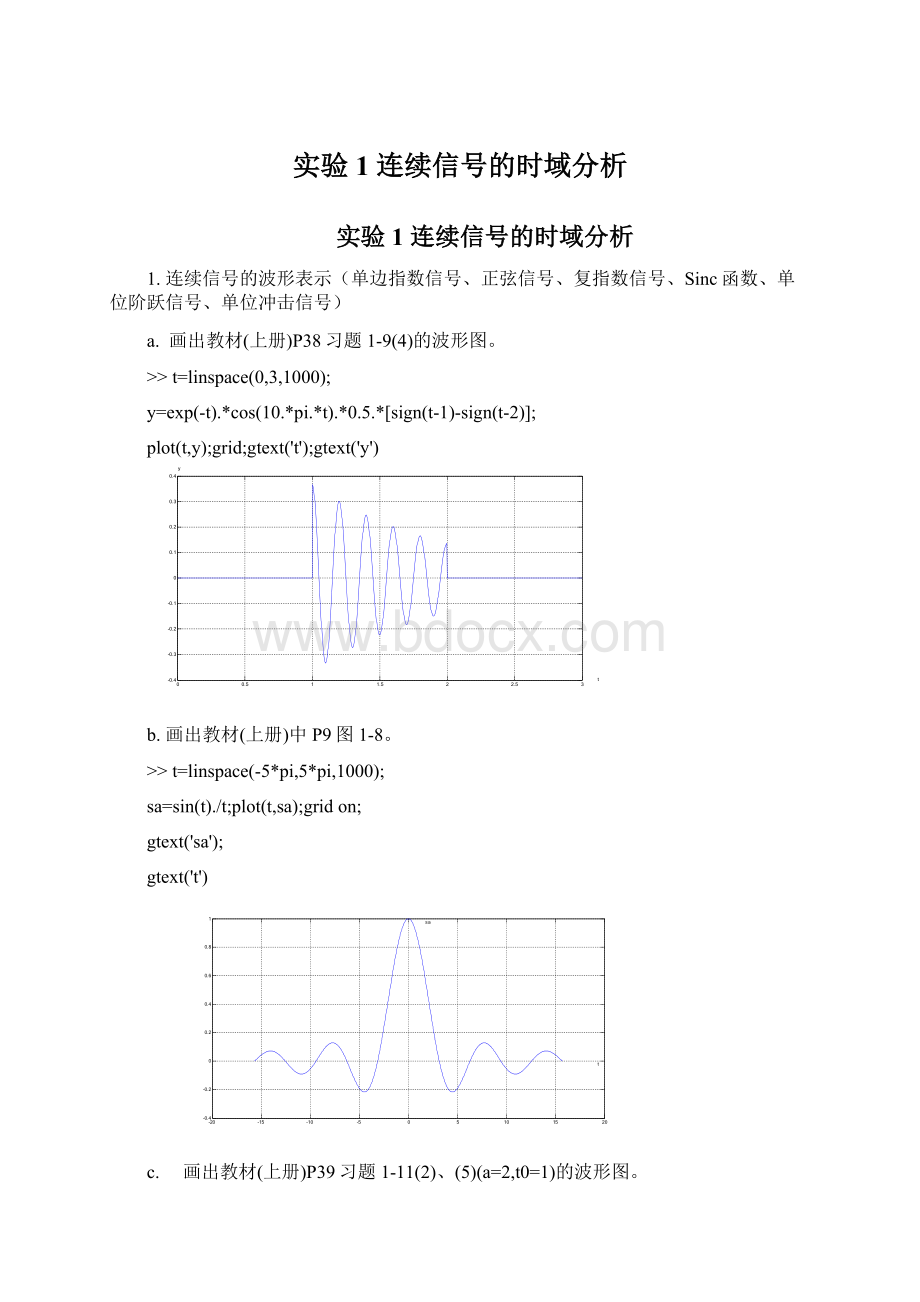
b.画出教材（上册）中P9图1-8。

t=linspace（-5*pi,5*pi,1000）;

sa=sin（t）./t;

plot（t,sa）;

gridon;

sa'

c.　画出教材（上册）P39习题1-11

（2）、（5）（a=2,t0=1）的波形图。

t=0:

0.0001:

3;

f=exp（1-t）.*（t>

1）.*（t<

2）;

plot（t,f）;

gridon;

gtext（'

f'

p391-11

（2）,（5）（a=2,t0=1）

f=sin（2*t-2）./（2*t-2）;

plot（t,f）;

d.用符号函数sign画出单位阶跃信号u（t-2）的波形（-5<

t<

10）

y=0.5.*[sign（t-2）+1];

%sign为　符号函数，利用sgn（t）=2u（t）-1变换来的

%grid为　网格的意思

xlabel（'

ylabel（'

axis（[-5,10,-1,2]）;

%axis为　坐标轴的意思

e.单位冲击信号可看作是宽度为

，幅度为

的矩形脉冲，即t=t1处的冲击信号为

画出

t1=1的单位冲击信号。

t=-3:

0.001:

f=2*[heaviside（t-1）-heaviside（t-1.5）];

axis（[02-0.12.5]）;

grid;

f.画出复指数信号

当

（0<

10）的实部和虚部的波形图。

10;

s=0.5+j*10;

y=exp（s*t）;

subplot（121）;

plot（t,real（y））;

real（y）'

subplot（122）;

plot（t,imag（y））;

imag（y）'

2.信号的基本运算（相加、相乘、反折、移位、尺度变换）

a.画出教材（上册）中P13图1-16、1-17（取

）.

y=sin（2*t）+sin（16*t）;

plot（t,y）

t=-2:

2;

y=sin（2*t）.*sin（16*t）;

b.利用符号函数subs画出教材（上册）中P11图1-13（a）（b）（c）（d）,并与P38习题1-4进行对比。

p11u.m:

functionf=u（t）

f=0.5.*[sign（t）+1];

initialsignal.m

functionf=initialsignal（t）

f=u（t+2）-u（t）+（1-t）.*[u（t）-u（t-1）];

f=initialsignal（t）;

subplot（411）;

axis（[-3,3,-0.5,1.5]）;

f（t）'

f2=initialsignal（t-2）;

subplot（412）;

plot（t,f2）;

f（t-2）'

f3=initialsignal（3*t-2）;

subplot（413）;

plot（t,f3）;

f（3*t-2）'

f4=initialsignal（-3*t-2）;

subplot（414）;

plot（t,f4）;

f（-3*t-2）'

P38

f2=initialsignal（3*t）;

f（3*t）'

f3=initialsignal（-3*t）;

f（-3*t）'

3.信号的奇偶分解

利用符号函数subs画出教材（上册）中P40习题1-18（c）（d）的波形并画出信号的奇分量和偶分量的波形。

u.mfunctionf=u（t）

f1.mfunctiony=f1（t）

y=cos（pi/2*t）.*[u（t+1）-u（t-1）]-cos（pi/2*t）.*[u（t-1）-u（t-3）];

f2.mfunctiony=f2（t）

y=（1-t）.*[u（t）-u（t-2）];

subplot（231）;

y=f1（t）;

f1（t）'

subplot（232）;

y2=1/2.*[f1（t）+f1（-t）];

plot（t,y2）;

f1e（t）'

subplot（233）;

y3=1/2.*[f1（t）-f1（-t）];

plot（t,y3）;

f1o（t）'

subplot（234）;

y=f2（t）;

f2（t）'

subplot（235）;

y2=1/2.*[f2（t）+f2（-t）];

f2e（t）'

subplot（236）;

y3=1/2.*[f2（t）-f2（-t）];

f2o（t）'