信号与系统课后matlab作业.docx
《信号与系统课后matlab作业.docx》由会员分享,可在线阅读,更多相关《信号与系统课后matlab作业.docx(26页珍藏版)》请在冰豆网上搜索。
信号与系统课后matlab作业
M2-1
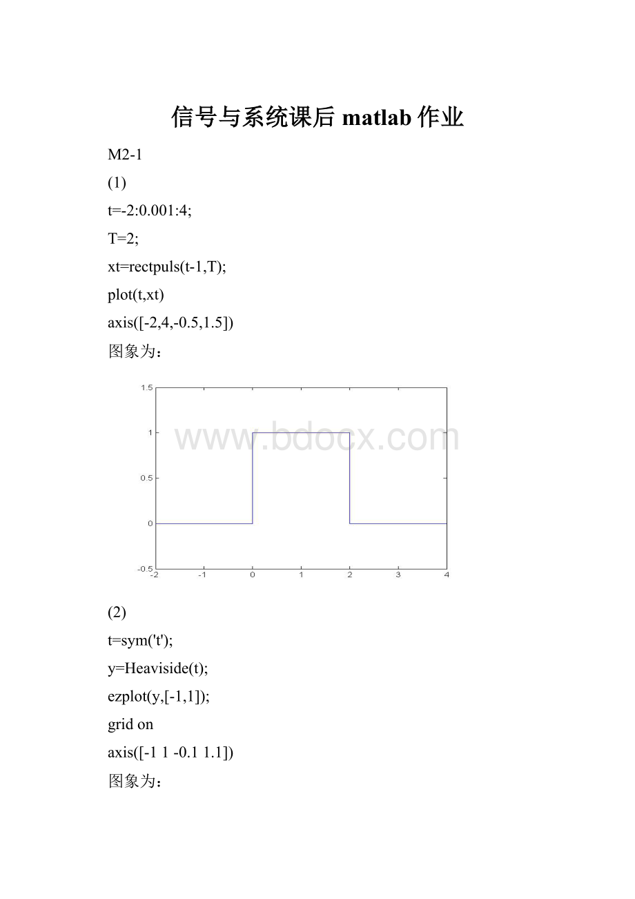
(1)
t=-2:
0.001:
4;
T=2;
xt=rectpuls(t-1,T);
plot(t,xt)
axis([-2,4,-0.5,1.5])
图象为:
(2)
t=sym('t');
y=Heaviside(t);
ezplot(y,[-1,1]);
gridon
axis([-11-0.11.1])
图象为:
(3)
A=10;a=-1;B=5;b=-2;
t=0:
0.001:
10;
xt=A*exp(a*t)-B*exp(b*t);
plot(t,xt)
图象为:
(4)
t=sym('t');
y=t*Heaviside(t);
ezplot(y,[-1,3]);
gridon
axis([-13-0.13.1])
图象为:
(5)
A=2;w0=10*pi;phi=pi/6;
t=0:
0.001:
0.5;
xt=abs(A*sin(w0*t+phi));
plot(t,xt)
图象为:
(6)
A=1;w0=1;B=1;w1=2*pi;
t=0:
0.001:
20;
xt=A*cos(w0*t)+B*sin(w1*t);
plot(t,xt)
图象为:
(7)
A=4;a=-0.5;w0=2*pi;
t=0:
0.001:
10;
xt=A*exp(a*t).*cos(w0*t);
plot(t,xt)
图象为:
(8)
w0=30;
t=-15:
0.001:
15;
xt=cos(w0*t).*sinc(t/pi);
plot(t,xt)
axis([-15,15,-1.1,1.1])
图象为:
M2-3
(1)functionyt=x2_3(t)
yt=(t).*(t>=0&t<=2)+2*(t>=2&t<=3)-1*(t>=3&t<=5);
(2)functionyt=x2_3(t)
yt=(t).*(t>=0&t<=2)+2*(t>=2&t<=3)-1*(t>=3&t<=5);
t=0:
0.001:
6;
subplot(3,1,1)
plot(t,x2_3(t))
title('x(t)')
axis([0,6,-2,3])
subplot(3,1,2)
plot(t,x2_3(0.5*t))
title('x(0.5t)')
axis([0,11,-2,3])
subplot(3,1,3)
plot(t,x2_3(2-0.5*t))
title('x(2-0.5t)')
axis([-6,5,-2,3])
图像为:
M2-9
(1)
k=-4:
7;
xk=[-3,-2,3,1,-2,-3,-4,2,-1,4,1,-1];
stem(k,xk,'file')
(2)
k=-12:
21;
x=[-3,0,0,-2,0,0,3,0,0,1,0,0,-2,0,0,-3,0,0,-4,0,0,2,0,0,-1,0,0,4,0,0,1,0,0,-1];
subplot(2,1,1)
stem(k,x,'file')
title('3倍内插')
t=-1:
2;
y=[-2,-2,2,1];
subplot(2,1,2)
stem(t,y,'file')
title('3倍抽取')
axis([-3,4,-4,4])
(3)
k=-4:
7;
x=[-3,-2,3,1,-2,-3,-4,2,-1,4,1,-1];
subplot(2,1,1)
stem(k+2,x,'file')
title('x[k+2]')
subplot(2,1,2)
stem(k-4,x,'file')
title('x[k-4]')
(4)
k=-4:
7;
x=[-3,-2,3,1,-2,-3,-4,2,-1,4,1,-1];
stem(-fliplr(k),fliplr(x),'file')
title('x[-k]')
M3-1
(1)
ts=0;te=5;dt=0.01;
sys=tf([21],[132]);
t=ts:
dt:
te;
x=exp(-3*t);
y=lsim(sys,x,t);
plot(t,y)
xlabel('Time(sec)')
ylabel('y(t)')
(2)
ts=0;te=5;dt=1;
sys=tf([21],[132]);
t=ts:
dt:
te;
x=exp(-3*t);
y=lsim(sys,x,t)
y=
0
0.6649
-0.0239
-0.0630
-0.0314
-0.0127
从
(1)
(2)对比我们当抽样间隔越小时数值精度越高。
M3-4
x=[0.85,0.53,0.21,0.67,0.84,0.12];
kx=-2:
3;
h=[0.68,0.37,0.83,0.52,0.71];
kh=-1:
3;
y=conv(x,h);
k=kx
(1)+kh
(1):
kx(end)+kh(end);
stem(k,y,'file');
M3-8
k=0:
30;
a=[10.7-0.45-0.6];
b=[0.8-0.440.360.02];
h=impz(b,a,k);
stem(k,h,'file')
M4-1
(1)对于周期矩形信号的傅里叶级数cn=-1/2j*sin(n/2*pi)*sinc(n/2)
n=-15:
15;
X=-j*1/2*sin(n/2*pi).*sinc(n/2);
subplot(2,1,1);
stem(n,abs(X),'file');
title('幅度谱')
xlabel('nw');
subplot(2,1,2);
stem(n,angle(X),'file');
title('相位谱')
(2)对于三角波信号的频谱是:
Cn=-
+
+
n=-15:
15;
X=sinc(n)-0.5*((sinc(n/2)).^2);
subplot(2,1,1);
stem(n,abs(X),'file');
title('幅度谱')
xlabel('nw');
subplot(2,1,2);
stem(n,angle(X),'file');
title('相位谱')
M4-6(4)
x=[1,2,3,0,0];
X=fft(x,5);
subplot(2,1,1);
m=0:
4;
stem(m,real(X),'file');
title('X[m]实部')
subplot(2,1,2);
stem(m,imag(X),'file');
title('X[m]虚部')
M4-7(3)
k=0:
10;
x=0.5.^k;
subplot(3,1,1);
stem(k,x,'file')
title('x[k]')
X=fft(x,10);
subplot(3,1,2);
m=0:
9;
stem(m,real(X),'file');
title('X[m]实部')
subplot(3,1,3);
stem(m,imag(X),'file');
title('X[m]虚部')
M5-2
t=0:
0.05:
2.5;
T=1;
xt1=rectpuls(t-0.5,T);
subplot(2,2,1)
plot(t,xt1)
title('x(t1)')
axis([0,2.5,0,2])
xt2=tripuls(t-1,2);
subplot(2,2,2)
plot(t,xt2)
title('x(t2)')
axis([0,2.5,0,2])
xt=xt1+xt2.*cos(50*t);
subplot(2,2,[3,4])
plot(t,xt)
title('x(t)')
figure;
b=[10000];
a=[1,26.131,341.42,2613.1,10000];
w=linspace(0,2*pi,200);
[H,w]=freqs(b,a,w);
subplot(2,1,1)
plot(w,abs(H));
title('幅度曲线')
subplot(2,1,2)
plot(w,angle(H));
title('相位曲线')
figure;
sys=tf([10000],[126.131341.422613.110000]);
yt1=lsim(sys,xt,t);
subplot(2,1,1);
plot(t,yt1);
title('y(t1)')
yt2=lsim(sys,xt.*cos(50*t),t);
subplot(2,1,2);
plot(t,yt2);
title('y(t2)')
M6-1
(1)
num=[41.6667];
den=[13.744425.760441.6667];
[r,p,k]=residue(num,den)
r=-0.9361-0.1895i-0.9361+0.1895i1.8722
p=-0.9361+4.6237i-0.9361-4.6237i-1.8722
k=[]
(2)
num=[1600];
den=[15.65698162262.7160000];
[r,p,k]=residue(num,den)
r=0.0992-1.5147i0.0992+1.5147i-0.0992+1.3137i-0.0992-1.3137i
p=-1.5145+21.4145i-1.5145-21.4145i-1.3140+18.5860i-1.3140-18.5860i
k=[]
(3)
num=[1000];
den=conv([15],[1525]);
[r,p,k]=residue(num,den)
r=-2.5000-1.4434i-2.5000+1.4434i-5.0000
p=-2.5000+4.3301i-2.5000-4.3301i-5.0000
k=1
(4)
num=[833.3025];
den=conv([14.112328.867],[19.927928.867]);
[r,p,k]=residue(num,den)
r=-2.4819+1.0281i-2.4819-1.0281i2.4819-5.9928i2.4819+5.9928i
p=-2.0562+4.9638i-2.0562-4.9638i-4.9640+2.0558i-4.9640-2.0558i
k=[]
M6-2
sys=tf(b,a);
x=1*(t>0)+0*(t<=0);
y1=lsim(sys,x,t);
plot(t,y1);
title('零状态响应')
figure;
[ABCD]=tf2ss(b,a);
sys=ss(A,B,C,D);
x=1*(t>0)+0*(t<=0);zi=[12];
y=lsim(sys,x,t,zi);
plot(t,y);
title('完全响应')
figure;
y2=y-y1;
plot(t,y2);
title('零输入响应')
M6-5
a=[1221];
b=[12];
sys=tf(b,a);
pzmap(sys)
冲击响应
a=[1221];
b=[12];
sys=tf(b,a);
impulse(sys)
阶跃响应
a=[1221];
b=[12];
sys=tf(b,a);
step(sys)
频率响应
a=[1221];
b=[12];
w=linspace(-10,10,20000);
H=freqs(b,a,w);
plot(w,abs(H))
M7-1
(1)
num=[216445632];
den=[33-1518-12];
[r,p,k]=residuez(num,den)
r=-0.01779.4914-3.0702+2.3398i-3.0702-2.3398i
p=-3.23611.23610.5000+0.8660i0.5000-0.8660i
k=-2.6667
(2)
num=[4-8.86-17.9826.74-8.04];
den=[1-210665];
[r,p,k]=residuez(num,den)
r=1.0849+1.3745i1.0849-1.3745i0.9769-1.2503i0.9769+1.2503i
p=2.0000+3.0000i2.0000-3.0000i-1.0000+2.0000i-1.0000-2.0000i
k=-0.1237
M7-2
k=0:
10;
a=[2-13];
b=[2-1];
y1=filter(b,a,x);
stem(k,y1)
title('零状态响应')
figure;
h=impz(b,a,k);
x=0.5.^k;
y2=conv(x,h);
N=length(y2);
stem(0:
N-1,y2)
title('零输入响应')
完全响应
y=y1+y2
M7-3
(1)
num=[216445632];
den=[33-1518-12];
zplane(num,den)
由图可知极点不是都在单位圆内,所以系统不是稳定系统。
(2)
num=[4-8.68-17.9826.74-8.04];
den=[1-210665];
zplane(num,den)
由图可知极点不是都在单位圆内,所以系统不是稳定系统。
 升级会员
升级会员 