机械原理第三章作业315.docx

机械原理第三章作业315.docx

《机械原理第三章作业315.docx》由会员分享，可在线阅读，更多相关《机械原理第三章作业315.docx（17页珍藏版）》请在冰豆网上搜索。

机械原理第三章作业315

平面连杆机构运动学分析

3-15

已知：

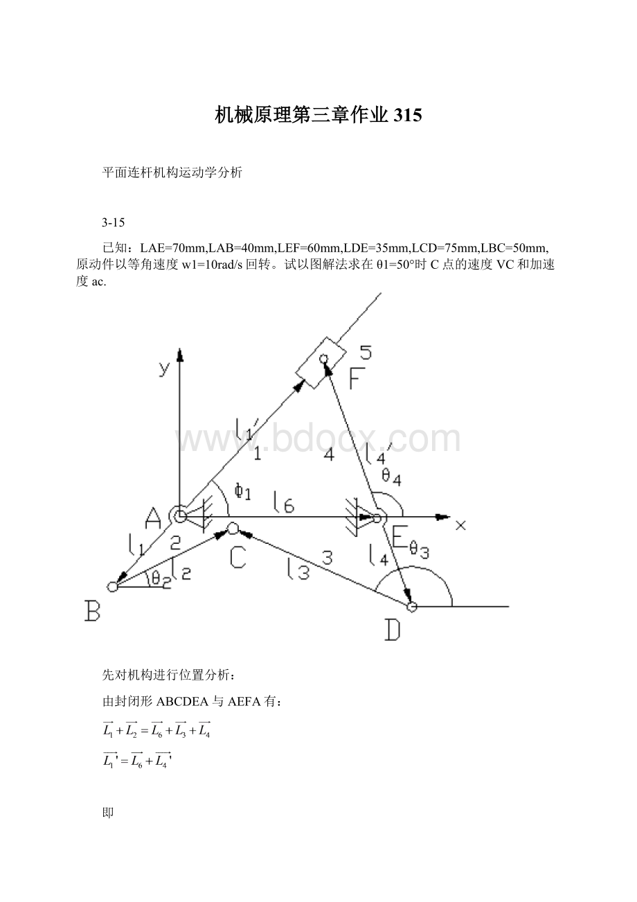
LAE=70mm,LAB=40mm,LEF=60mm,LDE=35mm,LCD=75mm,LBC=50mm,原动件以等角速度w1=10rad/s回转。

试以图解法求在θ1=50°时C点的速度VC和加速度ac.

先对机构进行位置分析：

由封闭形ABCDEA与AEFA有：

即

（1）

（2）

（1）位置方程中由1式可得：

（3）

由2式可得

（4）

解得

（5）

（2）速度方程

=

（6）

解得

（7）

（3）加速度方程

（8）

解得：

（9）

注意到，关于位置的四个方程组成的方程组是关于三角函数的非线性超越方程。

这里用牛顿——辛普森方法来求解。

第一步对位置方程进行求解：

首先用CAD对机构中AF杆的上极限位置进行分析，如图：

经理论验证，此时

，则：

下极限同理：

得出AF杆的运动范围是-58.9973°≤θ1≤58.9973°。

根据位置方程式编制如下rrrposi.m函数：

functiony=rrrposi（x）

%

%scriptusedtoimplementNewton-Raphsonmechodfor

%solvingnonlinearpositionofRRRbargroup

%

%Inputparameters

%x

（1）=theta-1

%x

（2）=theta-2guessvalue

%x（3）=theta-3guessvalue

%x（4）=theta-4guessvalue

%x（5）=l1

%x（6）=l2

%x（7）=l3

%x（8）=l4

%x（9）=l6

%x（10）=lAguessvalue

%x（11）=lB

%

%Outputparameters

%

%y

（1）=lA

%y

（2）=theta-2

%y（3）=theta-3

%y（4）=theta-4

%

theta2=x

（2）;

theta3=x（3）;

theta4=x（4）;

lA=x（10）

%

epsilon=1.0E-6;

%

f=[x（6）*cos（theta2）-x（7）*cos（theta3）-x（8）*cos（pi+theta4）+x（5）...

*cos（x

（1）+pi）-x（9）;

x（6）*sin（theta2）-x（7）*sin（theta3）-x（8）*sin（theta4+pi）+...

x（5）*sin（x

（1）+pi）;

-x（11）*cos（theta4）+lA*cos（x

（1））-x（9）;

-x（11）*sin（theta4）+lA*sin（x

（1））];

%

whilenorm（f）>epsilon

J=[0-x（6）*sin（theta2）x（7）*sin（theta3）-x（8）*sin（theta4）;

0x（6）*cos（theta2）-x（7）*cos（theta3）x（8）*cos（theta4）;

cos（x

（1））00x（11）*sin（theta4）;

sin（x

（1））00-x（11）*cos（theta4）];

dth=inv（J）*（-1.0*f）;

lA=lA+dth

（1）;

theta2=theta2+dth

（2）;

theta3=theta3+dth（3）;

theta4=theta4+dth（4）;

f=[x（6）*cos（theta2）-x（7）*cos（theta3）-x（8）*cos（pi+theta4）+x（5）...

*cos（x

（1）+pi）-x（9）;

x（6）*sin（theta2）-x（7）*sin（theta3）-x（8）*sin（theta4+pi）+...

x（5）*sin（x

（1）+pi）;

-x（11）*cos（theta4）+lA*cos（x

（1））-x（9）;

-x（11）*sin（theta4）+lA*sin（x

（1））];

norm（f）;

end;

y

（1）=lA;

y

（2）=theta2;

y（3）=theta3;

y（4）=theta4;

再进行数据输入，运行程序进行运算。

这里我们根据上面分析的θ1的极限位置取θ1的范围为40°~55°并均分成15个元素：

clc

clear

x1=linspace（40*pi/180,55*pi/180,15）;%linspace（a,b,n）在区间[a,b]中均匀取n个点

x=zeros（length（x1）,118）;%length是求某一矩阵所有维的最大长度

forn=1:

15

x（n,:

）=[x1（:

n）pi/68*pi/92*pi/340507535707560];

end

p=zeros（length（x1）,4）;

fork=1:

15

y=rrrposi（x（k,:

））;

p（k,:

）=y;

end

>>p

p=

93.31490.71632.54551.5461

91.30710.70452.56171.5902

89.23870.69292.57861.6347

87.10760.68152.59631.6796

84.91130.67032.61471.7250

82.64630.65922.63391.7709

80.30860.64822.65391.8174

77.89310.63722.67471.8646

75.39300.62632.69651.9126

72.79980.61542.71921.9616

70.10190.60432.74312.0118

67.28330.59302.76832.0635

64.32170.58122.79502.1169

61.18350.56872.82372.1728

57.81530.55512.85492.2319

输出的P、矩阵的第二列到第四列分别是θ2、θ3、θ4的值，第一列是AF杆的长度L1’。

第二步进行速度计算：

根据速度方程式编写如下rrrvel.m函数：

functiony=rrrvel（x）

%

%Inputparameters

%

%x

（1）=theta-1

%x

（2）=theta-2

%x（3）=theta-3

%x（4）=theta-4

%x（5）=dtheta-1

%x（6）=l1

%x（7）=l2

%x（8）=l3

%x（9）=l4

%x（10）=l6

%x（11）=lA

%x（12）=lB

%

%Outoutparameters

%

%y

（1）=V

%y

（2）=dtheta-2

%y（3）=dtheta-3

%y（4）=dtheta-4

%

A=[-x（7）*sin（x

（2））x（8）*sin（x（3））x（9）*sin（pi+x（4））0;

x（7）*cos（x

（2））-x（8）*cos（x（3））-x（9）*cos（x（4）+pi）0;

00x（12）*sin（x（4））cos（x

（1））;

00-x（12）*cos（x（4））sin（x

（1））];

B=[x（6）*sin（x

（1）+pi）;-x（6）*cos（x

（1）+pi）;x（11）*sin（x

（1））;-x（11）*cos（x

（1））]*x（5）;

y=inv（A）*B;

根据第一步得到的数据进行数据输入，运行程序计算各速度值。

程序如下：

x2=[x1'p（:

2）p（:

3）p（:

4）10*ones（15,1）40*ones（15,1）50*ones（15,1）...

75*ones（15,1）35*ones（15,1）70*ones（15,1）p（:

1）60*ones（15,1）];

q=zeros（4,15）;

form=1:

15

y2=rrrvel（x2（m,:

））;

q（:

m）=y2;

end

q=

1.0e+003*

Columns1through8

-0.0064-0.0062-0.0061-0.0061-0.0060-0.0059-0.0059-0.0058

0.00850.00890.00920.00960.01010.01050.01090.0114

0.02350.02370.02390.02410.02440.02470.02500.0255

-1.0578-1.0897-1.1226-1.1568-1.1926-1.2302-1.2704-1.3137

Columns9through15

-0.0058-0.0059-0.0060-0.0062-0.0065-0.0069-0.0078

0.01190.01250.01310.01390.01480.01590.0175

0.02590.02650.02720.02810.02920.03060.0327

-1.3610-1.4136-1.4734-1.5431-1.6273-1.7337-1.8767

程序运行得到q矩阵，第一行到第三行分别是a2、a3、a4的值，第四行是杆AF上滑块运动的速度，即F点的速度。

第三步进行加速度计算：

编写加速度计算函数rrra.m：

functiony=rrra（x）

%

%Inputparameters

%

%x

（1）=th1

%x

（2）=th2

%x（3）=th3

%x（4）=th4

%x（5）=dth1

%x（6）=dth2

%x（7）=dth3

%x（8）=dth4

%x（9）=r1

%x（11）=r3

%x（12）=r4

%x（13）=r6

%x（14）=lA

%x（15）=lB

%x（16）=V

%

%y

（1）=ddth2

%y

（2）=ddth3

%y（3）=ddth4

%y（4）=a

%

A=[-x（10）*sin（x

（2））x（11）*sin（x（3））-x（14）*sin（x（4））0;

x（10）*cos（x

（2））-x（11）*cos（x（3））x（14）*cos（x（4））0;

00x（15）*sin（x（4））cos（x

（1））;

00-x（15）*cos（x（4））sin（x

（1））];

B=[-x（10）*x（6）*cos（x

（2））x（11）*x（7）*cos（x（3））-x（12）*x（8）*cos（x（4））0;

-x（10）*x（6）*sin（x

（2））-x（11）*x（7）*sin（x（3））-x（12）*x（8）*sin（x（4））0;

00x（15）*x（8）*cos（x（4））-x（5）*sin（x

（1））;

00x（15）*x（8）*sin（x（4））x（5）*cos（x

（1））];

C=[x（6）;x（7）;x（8）;x（16）];

D=[x（9）*x（5）*cos（x

（1））;x（9）*x（5）*sin（x

（1））;x（14）*x（5）*cos（x

（1））+x（16）*sin（x

（1））;x（14）*x（5）*sin（x

（1））-x（16）*cos（x

（1））];

y=inv（A）*D-inv（A）*B*C;

根据第一步和第二步输入数据，运行程序得到各加速度的值：

x3=[x1'p（:

2）p（:

3）p（:

4）10*ones（15,1）q（1,:

）'q（2,:

）'q（3,:

）'...

40*ones（15,1）50*ones（15,1）75*ones（15,1）35*ones（15,1）70*ones（15,1）p（:

1）...

60*ones（15,1）q（4,:

）'];

f=zeros（4,15）;

form=1:

15

y3=rrra（x3（m,:

））;

f（:

m）=y3;

end

>>f

f=

1.0e+005*

Columns1through8

-0.0038-0.0040-0.0042-0.0044-0.0047-0.0050-0.0054-0.0058

0.00600.00640.00680.00720.00770.00830.00890.0097

0.00330.00360.00390.00420.00460.00500.00560.0062

-0.3601-0.3723-0.3866-0.4033-0.4231-0.4468-0.4755-0.5107

Columns9through15

-0.0064-0.0071-0.0081-0.0094-0.0112-0.0139-0.0185

0.01060.01170.01310.01500.01760.02140.0276

0.00700.00800.00930.01100.01340.01710.0231

-0.5548-0.6111-0.6851-0.7857-0.9290-1.1462-1.5071

接下来计算C点在θ1=55°，w1=10rad/s时的速度，加速度：

Vx=40*10*sin（55）-50*q（1,10）*sin（p（10,2））;

Vy=40*10*cos（55）+50*q（1,10）*cos（p（10,2））;

ax=100*40*cos（50）-q（1,10）^2*50*cos（p（10,2））-f（1,10）*50*sin（p（10,2））;

ay=100*40*cos（50）-q（1,10）^2*50*cos（p（10,2））-f（1,10）*50*sin（p（10,2））;

输出结果：

Vx=-230.2208;Vy=-231.1533;

ax=2.3069e+004;ay=2.3069e+004;

表1各构件的位置、速度和加速度

θ1

θ2

θ3

θ4

L1’

W2

W3

W4

V

a2

a2

a2

al

rad

mm

rad/s

mm/s

x10^3

rad/s^2

x10^3

mm/s^2

x10^5

0.6981

0.7168

0.7355

0.7542

0.7729

0.7916

0.8103

0.8290

0.8477

0.8664

0.8851

0.9038

0.9225

0.9412

0.9599

0.7163

0.7045

0.6929

0.6815

0.6703

0.6592

0.6482

0.6372

0.6263

0.6154

0.6043

0.5930

0.5812

0.5687

0.5551

2.5455

2.5617

2.5786

2.5963

2.6147

2.6339

2.6539

2.6747

2.6965

2.7192

2.7431

2.7683

2.7950

2.8237

2.8549

1.5461

1.5902

1.6347

1.6796

1.7250

1.7709

1.8174

1.8646

1.9126

1.9616

2.0118

2.0635

2.1169

2.1728

2.2319

93.3149

91.3071

89.2387

87.1076

84.9113

82.6463

80.3086

77.8931

75.3930

72.7998

70.1019

67.2833

64.3217

61.1835

57.8153

-6.3578

-6.2487

-6.1469

-6.0541

-5.9726

-5.9054

-5.8561

-5.8299

-5.8340

-5.8786

-5.9789

-6.1587

-6.4572

-6.9440

-7.7555

8.4725

8.8575

9.2469

9.6433

10.0502

10.4720

10.9145

11.3856

11.8957

12.4601

13.1005

13.8507

14.7646

15.9364

17.5470

23.5099

23.6948

23.9018

24.1350

24.3994

24.7013

25.0491

25.4538

25.9305

26.5003

27.1937

28.0569

29.1637

30.6408

32.7288

-1.0578

-1.0897

-1.1226

-1.1568

-1.1926

-1.2302

-1.2704

-1.3137

-1.3610

-1.4136

-1.4734

-1.5431

-1.6273

-1.7337

-1.8767

-0.3790

-0.3960

-0.4156

-0.4386

-0.4656

-0.4976

-0.5361

-0.5829

-0.6409

-0.7144

-0.8099

-0.9386

-1.1206

-1.3948

-1.8491

0.6037

0.6395

0.6788

0.7225

0.7715

0.8274

0.8919

0.9677

1.0587

1.1707

1.3128

1.4999

1.7586

2.1406

2.7600

0.3334

0.3590

0.3879

0.4210

0.4592

0.5038

0.5567

0.6205

0.6989

0.7976

0.9255

1.0976

1.3402

1.7052

2.3084

-0.3601

-0.3723

-0.3866

-0.4033

-0.4231

-0.4468

-0.4755

-0.5107

-0.5548

-0.6111

-0.6851

-0.7857

-0.9290

-1.1462

-1.5071

接下来输出图像：

角位置图像，程序如下

plot（x1,p（:

2）,'--',x1,p（:

3）,':

',x1,p（:

4）,'*'）

title（'角位置'）;

xlabel（'\theta1/rad'）;

ylabel（'\theta2、\theta3、\theta4/rad'）;

输出图像如图：

AF长度图像，程序如下：

plot（x1,p（:

1））

xlabel（'\theta1/rad'）;

ylabel（'L1''/mm'）;

输出图像如下：

角速度：

plot（x1,q（1,:

）,'--',x1,q（2,:

）,':

',x1,q（3,:

）,'*'）

xlabel（'W1rad/s'）;

ylabel（'W2、W3、W4rad/S'）;

title（'角速度'）;

F点速度：

plot（x1,q（4,:

））

xlabel（'W1rad/s'）;

ylabel（'Vmm/s'）;

title（'F点速度'）;

角加速度：

plot（x1,f（1,:

）,'--',x1,f（2,:

）,':

',x1,f（3,:

）,'*'）

xlabel（'W1rad/s'）;

ylabel（'\alpha2、\alpha3、\alpha4rad/S^2'）;

title（'角加速度'）;

F点的加速度：

plot（x1,f（4,:

））

xlabel（'W1rad/s'）;

ylabel（'amm/s^2'）;

title（'F点的加速度'）;

任务分配：

1.收集资料：

严日明刘德亭

2.计算分析：

严日明

3．编程：

严日明刘德亭

4．编辑工作：

刘德亭

5．校核：

严日明刘德亭

参考文献

【1】孙恒，陈作模.机械原理【M】.7版.北京：

高等教育出版社，2006

【2】曲秀全.基于MATLAB/Simulink平面连杆机构的动态仿真.黑龙江：

哈尔滨工业大学出版社，2007

【3】高会生，李新叶，胡志奇译.MATLAB原理与工程应用.2版.北京：

电子工业出版社，2006

【4】贺超英.MATLAB应用与实验教程.北京：

电子工业出版社，2010

【5】王宏.MATLAB6.5及其在信号处理中的应用.北京：

清华大学出版社，2004

【6】同济大学数学系.线性代数.北京：

高等教育出版社，2009

【7】同济大学数学系.高等数学.北京：

高等教育出版社，2008

【8】雷培，刘云霞.基于MATLAB的四连杆机构运动分析.机械工程与自动化.2009年4月，第2期

【9】李团结，贾建援，胡雪梅.机械工程中两类非线性方程组的完全解.西安电子科技大学学报（自然科学版）2005年2月，第32卷，第1期

【10】董长虹，余海啸.MATLAB接口技术与应用.北京：

国防工业出版社，2004

【11】周品，何正风.MATLAB数值分析.北京：

机械工业出版社，2009