东华大学信号报告13.docx
《东华大学信号报告13.docx》由会员分享,可在线阅读,更多相关《东华大学信号报告13.docx(20页珍藏版)》请在冰豆网上搜索。
东华大学信号报告13
1.1
>>t=-4:
0.001:
4;
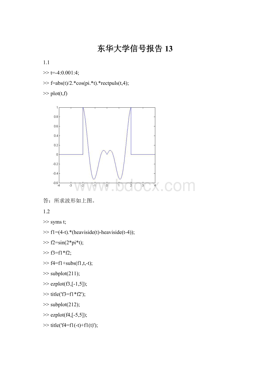
>>f=abs(t)/2.*cos(pi.*t).*rectpuls(t,4);
>>plot(t,f)
答:
所求波形如上图。
1.2
>>symst;
>>f1=(4-t).*(heaviside(t)-heaviside(t-4));
>>f2=sin(2*pi*t);
>>f3=f1*f2;
>>f4=f1+subs(f1,t,-t);
>>subplot(211);
>>ezplot(f3,[-1,5]);
>>title('f3=f1*f2');
>>subplot(212);
>>ezplot(f4,[-5,5]);
>>title('f4=f1(-t)+f1(t)');
1.3
>>t=-10:
0.001:
10;
>>f=1+cos(pi/4.*t-pi/3)+2*cos(t.*pi/2-pi/4)+cos(2*pi.*t);
>>plot(t,f)
>>y=@(t)1+cos(pi/4.*t-pi/3)+2*cos(t.*pi/2-pi/4)+cos(2*pi.*t);
>>[Xmin1,Ymin1]=fminbnd(y,-2,-1)
Xmin1=
-1.5139
Ymin1=
-2.6131
>>[Xmin2,Ymin2]=fminbnd(y,6,7)
Xmin2=
6.4861
Ymin2=
-2.6131
>>T=Xmin2-Xmin1
T=
8.0000
答:
由f1波形知该信号是周期函数,周期为8
1.4
>>b=[1];
>>a=[116];
>>sys=tf(b,a);
>>t=0:
0.01:
0.5;
>>x=exp(-1.*t);
>>lsim(sys,x,t)
>>y=lsim(sys,x,t)
y=
0
0.0000
0.0002
0.0004
0.0008
0.0012
0.0017
0.0023
0.0030
0.0038
0.0047
0.0056
0.0066
0.0077
0.0088
0.0101
0.0114
0.0127
0.0141
0.0156
0.0172
0.0188
0.0204
0.0221
0.0239
0.0257
0.0275
0.0294
0.0313
0.0333
0.0353
0.0373
0.0394
0.0414
0.0436
0.0457
0.0479
0.0500
0.0522
0.0544
0.0567
0.0589
0.0611
0.0634
0.0656
0.0679
0.0702
0.0724
0.0747
0.0769
0.0791
0.0814
0.0836
0.0858
0.0880
0.0902
1.5
M文件“sconv.m”代码:
function[fc,t]=sconv(f1,f2,t1,t2,dt)
fc=conv(f1,f2);
fc=fc.*dt;
t0=t1
(1)+t2
(1);
l=length(f1)+length(f2)-2;
t=t0:
dt:
(t0+l.*dt);
命令窗口:
ts=-4;
te=4;
dt=0.001;
t=ts:
dt:
te;
t1=t;
t2=t;
f=0.5*t;
f1=2*(heaviside(t+1)-heaviside(t-1));
f2=heaviside(t+2)-heaviside(t-2);
[fc,t]=sconv(f1,f2,t1,t2,dt);
plot(t,fc);
axis([-44-26]);
xlabel(‘t’);
title(‘'f1(t)与f2(t)卷积积分’);
心得总结:
初步尝试门函数rectpuls的使用。
了解到用heaviside函数表示门函数,为了表示函数f(-t),大致了解了换元函数subs的使用。
加深了对内联函数的理解,为了求函数周期,知悉了利用函数fminbnd结合函数图形求局部最小值的方法。
初步了解用函数lsim求系统零状态响应的大致方法。
掌握用M文件计算卷积积分的方法,加深了对M文件概念的理解。
2.2
(1)
M文件“fouri2.m”:
functiony=fouri2(A,t,tao)
f=(A*(heaviside(t+tao/2)-heaviside(t-tao/2)));
y=fourier(f);
ezplot(abs(y),[-6*pi,6*pi]);
axis([-2020-0.210]);
gridon;
xlabel('\omega');
ylabel('Magnitude');
title('|F(j\omega)|');
命令窗口:
>>symst;
>>f1=fouri2(2,t,4)
f1=
-2*exp(-w*2*i)*(pi*dirac(w)-i/w)+2*exp(w*2*i)*(pi*dirac(w)-i/w)
>>f2=fouri2(2,t,6)
f2=
-2*exp(-w*3*i)*(pi*dirac(w)-i/w)+2*exp(w*3*i)*(pi*dirac(w)-i/w)
>>f3=fouri2(2,t,20)
f3=
-2*exp(-w*10*i)*(pi*dirac(w)-i/w)+2*exp(w*10*i)*(pi*dirac(w)-i/w)
>>f4=fouri2(2,t,20)
f4=
-2*exp(-w*10*i)*(pi*dirac(w)-i/w)+2*exp(w*10*i)*(pi*dirac(w)-i/w)
2.2
(2)
M文件“fouri22.m”:
functiony=fouri22(A,t,tao)
f=(A*(heaviside(t+tao/2)-heaviside(t-tao/2)));
y=fourier(f);
subplot(121);
ezplot(f,[-6*pi,6*pi]);
gridon;
xlabel('t');
ylabel('f(t)');
subplot(122);
ezplot(abs(y),[-6*pi,6*pi]);
axis([-2020-0.11.1]);
gridon;
xlabel('\omega');
ylabel('Magnitude');
title('|F(j\omega)|');
命令窗口:
>>symst;
>>f21=fouri22(1,t,1)
f21=
(cos(w/2)*i+sin(w/2))/w-(cos(w/2)*i-sin(w/2))/w
>>f22=fouri22(0.5,t,2)
f22=
-(exp(-w*i)*(pi*dirac(w)-i/w))/2+(exp(w*i)*(pi*dirac(w)-i/w))/2
>>f23=fouri22(0.1,t,10)
f23=
-(exp(-w*5*i)*(pi*dirac(w)-i/w))/10+(exp(w*5*i)*(pi*dirac(w)-i/w))/10
2.3
(2)
>>b=[0.100];
>>a=[0.115];
>>[H,w]=freqs(b,a);
>>subplot(211);
>>plot(w,abs(H));
>>set(gca,'xtick',[0:
4:
100]);
>>set(gca,'ytick',[00.40.7071]);
>>xlabel('\omega');
>>ylabel('Magnitude');
>>title('|H(j\omega)|');
>>gridon;
>>subplot(212);
>>plot(w,angle(H));
>>set(gca,'xtick',[0:
4:
100]);
>>set(gca,'ytick',[00.40.7071]);
>>xlabel('\omega');
>>ylabel('Phase');
>>title('\phi(\omega)');
2.4
(1)
M文件“eg24.m”:
function[H,w]=eg24(RC)
b=[01];
a=[RC1];
[H,w]=freqs(b,a);
subplot(211);
plot(w,abs(H));
set(gca,'xtick',[0:
10]);
set(gca,'ytick',[00.40.7071]);
xlabel('\omega');
ylabel('Magnitude');
title('|H(j\omega)|');
gridon;
subplot(212);
plot(w,angle(H));
set(gca,'xtick',[0:
10]);
set(gca,'ytick',[00.40.7071]);
xlabel('\omega');
ylabel('Phase');
title('\phi(\omega)');
命令窗口:
>>[H1,w1]=eg24(0.001);
>>[H2,w2]=eg24(0.002);
>>[H3,w3]=eg24(0.003);
>>[H4,w4]=eg24(0.004);
>>[H5,w5]=eg24(0.01);
>>[H6,w6]=eg24(0.1);
2.4
(2)
symstw;
RC=1;
H=1/(RC*j*w+1);
e=cos(100*t)+cos(3000*t);
E=fourier(e);
R=E*H;
r=ifourier(R);
t1=0:
0.0001:
0.2;
e1=cos(100*t1)+cos(3000*t1);
subplot(221);
plot(t1,e1);
xlabel('t');
title('e=cos(100*t)+cos(3000*t)');
subplot(222);
ezplot(r,[00.2]);
xlabel('t');
title('r(t)');
gridon;
b=[01];
a=[RC1];
[H,w]=freqs(b,a);
subplot(223);
plot(w,abs(H));
set(gca,'xtick',[0:
10]);
set(gca,'ytick',[00.40.7071]);
xlabel('\omega');
ylabel('Magnitude');
title('|H(j\omega)|');
gridon;
subplot(224);
plot(w,angle(H));
set(gca,'xtick',[0:
10]);
set(gca,'ytick',[00.40.7071]);
xlabel('\omega');
ylabel('Phase');
title('\phi(\omega)');
gridon;
3.1
>>s=tf('s');
>>G=(1-s)/(1+s);
>>bode(G)
 升级会员
升级会员 