ch5可视化a.docx
《ch5可视化a.docx》由会员分享,可在线阅读,更多相关《ch5可视化a.docx(34页珍藏版)》请在冰豆网上搜索。
ch5可视化a
第5章数据和函数的可视化
.1引导
.1.1离散数据和离散函数的可视化
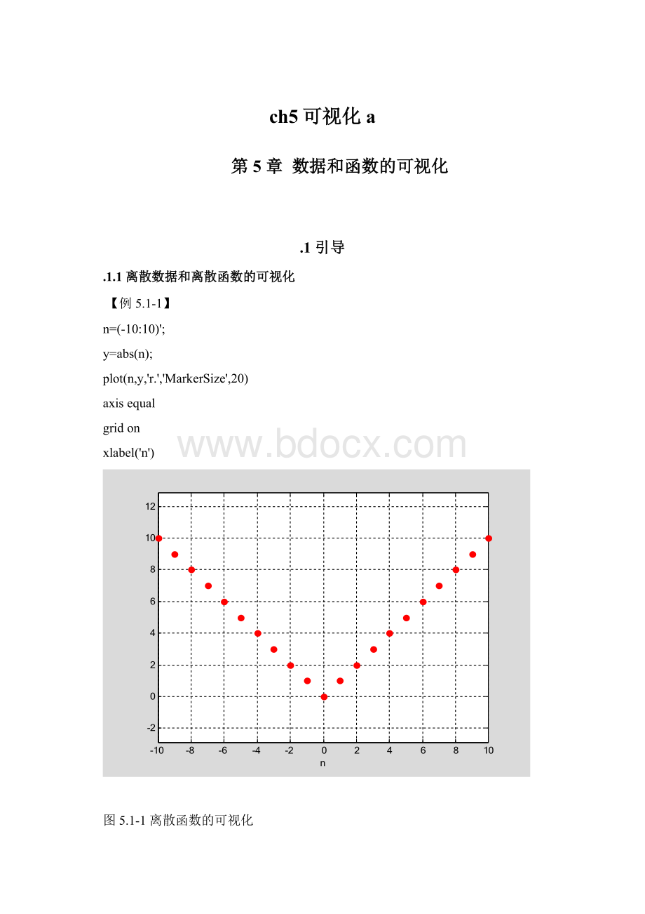
【例5.1-1】
n=(-10:
10)';
y=abs(n);
plot(n,y,'r.','MarkerSize',20)
axisequal
gridon
xlabel('n')
图5.1-1离散函数的可视化
.1.2连续函数的可视化
【例5.1-2】
t1=(0:
11)/11*pi;
t2=(0:
400)/400*pi;
t3=(0:
50)/50*pi;
y1=sin(t1).*sin(9*t1);
y2=sin(t2).*sin(9*t2);
y3=sin(t3).*sin(9*t3);
subplot(2,2,1),plot(t1,y1,'r.')
axis([0,pi,-1,1]),title('
(1)点过少的离散图形')
subplot(2,2,2),plot(t1,y1,t1,y1,'r.')
axis([0,pi,-1,1]),title('
(2)点过少的连续图形')
subplot(2,2,3),plot(t2,y2,'r.')
axis([0,pi,-1,1]),title('(3)点密集的离散图形')
subplot(2,2,4),plot(t3,y3)
axis([0,pi,-1,1]),title('(4)点足够的连续图形')
图5.1-2连续函数的图形表现方法
【例5.1-3】
N=9;
t=0:
2*pi/N:
2*pi;
x=sin(t);y=cos(t);
tt=reshape(t,2,(N+1)/2);
tt=flipud(tt);
tt=tt(:
);
xx=sin(tt);yy=cos(tt);
subplot(1,2,1),plot(x,y)
title('
(1)正常排序图形'),axisequaloff,shg
subplot(1,2,2),plot(xx,yy)
title('
(2)非正常排序图形'),axisequaloff,shg
图5.1-3自变量排列次序对连续曲线图形的影响
.2二维曲线和图形
.2.1二维曲线绘制的基本指令plot
【例5.2-1】
clf
t=(0:
pi/50:
2*pi)';
k=0.4:
0.1:
1;
Y=cos(t)*k;
subplot(1,2,1)
plot(t,Y,'LineWidth',1.5)
title('Byplot(t,Y)')
xlabel('t')
subplot(1,2,2)
plot(Y,'LineWidth',1.5)
title('Byplot(Y)')
xlabel('rowsubscriptofY')
图5.2-1plot(t,Y)与plot(Y)所绘曲线的区别
【例5.2-2】
t=(0:
pi/100:
pi)';
y1=sin(t)*[1,-1];
y2=sin(t).*sin(9*t);
t3=pi*(0:
9)/9;
y3=sin(t3).*sin(9*t3);
plot(t,y1,'r:
',t,y2,'-bo')
holdon
plot(t3,y3,'s','MarkerSize',10,'MarkerEdgeColor',[0,1,0],'MarkerFaceColor',[1,0.8,0])
axis([0,pi,-1,1])
holdoff
%plot(t,y1,'r:
',t,y2,'-bo',t3,y3,'s','MarkerSize',10,'MarkerEdgeColor',[0,1,0],'MarkerFaceColor',[1,0.8,0])
图5.2-2属性控制下所绘曲线
.2.2坐标控制和图形标识
【例5.2-3】
t=0:
2*pi/99:
2*pi;
x=1.15*cos(t);y=3.25*sin(t);
subplot(2,3,1),plot(x,y),axisnormal,gridon,
title('NormalandGridon')
subplot(2,3,2),plot(x,y),axisequal,gridon,title('Equal')
subplot(2,3,3),plot(x,y),axissquare,gridon,title('Square')
subplot(2,3,4),plot(x,y),axisimage,boxoff,title('ImageandBoxoff')
subplot(2,3,5),plot(x,y),axisimagefill,boxoff
title('ImageandFill')
subplot(2,3,6),plot(x,y),axistight,boxoff,title('Tight')
图5.2-3各种轴控制指令的不同影响
【例5.2-4】
clf;t=0:
pi/50:
2*pi;
y=sin(t);
plot(t,y)
axis([0,2*pi,-1.2,1.2])
text(pi/2,1,'\fontsize{16}\leftarrow\itsin(t)\fontname{隶书}极大值')
title('y=sin(t)')
xlabel('t')
ylabel('y')
图5.2-4试验标识的图形
【例5.2-5】
clf;t=6*pi*(0:
100)/100;
y=1-exp(-0.3*t).*cos(0.7*t);
plot(t,y,'r-','LineWidth',3)
holdon
tt=t(find(abs(y-1)>0.05));ts=max(tt);
plot(ts,0.95,'bo','MarkerSize',10)
holdoff
axis([-inf,6*pi,0.6,inf])
set(gca,'Xtick',[2*pi,4*pi,6*pi],'Ytick',[0.95,1,1.05,max(y)])
set(gca,'XtickLabel',{'2*pi';'4*pi';'6*pi'})
set(gca,'YtickLabel',{'0.95';'1';'1.05';'max(y)'})
gridon
text(13.5,1.2,'\fontsize{12}{\alpha}=0.3')
text(13.5,1.1,'\fontsize{12}{\omega}=0.7')
cell_string{1}='\fontsize{12}\uparrow';
cell_string{2}='\fontsize{16}\fontname{隶书}镇定时间';
cell_string{3}='\fontsize{6}';
cell_string{4}=['\fontsize{14}\rmt_{s}='num2str(ts)];
text(ts,0.85,cell_string,'Color','b','HorizontalAlignment','Center')
title('\fontsize{14}\ity=1-e^{-\alphat}cos{\omegat}')
xlabel('\fontsize{14}\bft\rightarrow')
ylabel('\fontsize{14}\bfy\rightarrow')
图5.2-5二阶阶跃响应图的标识
.2.3多次叠绘、双纵坐标和多子图
【例5.2-6】
t=2*pi*(0:
20)/20;
y=cos(t).*exp(-0.4*t);
stem(t,y,'g','Color','k');
holdon
stairs(t,y,':
r','LineWidth',3)
holdoff
legend('\fontsize{14}\itstem','\fontsize{14}\itstairs')
boxon
图5.2-6离散信号的重构
【例5.2-7】
clf;dx=0.1;x=0:
dx:
4;y=x.*sin(x);
s=cumtrapz(y)*dx;
a=plotyy(x,y,x,s,'stem','plot');
text(0.5,1.5,'\fontsize{14}\ity=xsinx')
sint='{\fontsize{16}\int_{\fontsize{8}0}^{x}}';
ss=['\fontsize{14}\its=',sint,'\fontsize{14}\itxsinxdx'];
text(2.5,3.5,ss)
set(get(a
(1),'Ylabel'),'String','被积函数\ity=xsinx')
set(get(a
(2),'Ylabel'),'String',ss)
xlabel('x')
图5.2-7函数和积分
【例5.2-8】
clf;t=(pi*(0:
1000)/1000)';
y1=sin(t);y2=sin(10*t);y12=sin(t).*sin(10*t);
subplot(2,2,1),plot(t,y1);axis([0,pi,-1,1])
subplot(2,2,2),plot(t,y2);axis([0,pi,-1,1])
subplot('position',[0.2,0.1,0.6,0.40])
plot(t,y12,'b-',t,[y1,-y1],'r:
')
axis([0,pi,-1,1])
图5.2-8多子图的布置
.2.4获取二维图形数据的指令ginput
【例5.2-9】
clf
x=0:
0.01:
1;
y=(x+2).^x-2;
plot(x,y);
gridon
图5.2-9经多次试探后画出的图形
图5.2-10局部放大图
[x,y]=ginput
(1);
formatlong
x,y
x=
0.69828692903537
y=
-5.884401711382421e-010
.3三维曲线和曲面
.3.1三维线图指令plot3
【例5.3-1】
t=(0:
0.02:
2)*pi;
x=sin(t);y=cos(t);z=cos(2*t);
plot3(x,y,z,'b-',x,y,z,'bd')
view([-82,58]),boxon
xlabel('x'),ylabel('y'),zlabel('z')
legend('链','宝石','Location','best')
图5.3-1宝石项链
.3.2三维曲面/网线图
【例5.3-2】
clf
x=-4:
4;y=x;
[X,Y]=meshgrid(x,y);
Z=X.^2+Y.^2;
surf(X,Y,Z);
colormap(hot)
holdon
stem3(X,Y,Z,'bo')
holdoff
xlabel('x'),ylabel('y'),zlabel('z')
axis([-5,5,-5,5,0,inf])
view([-84,21])
图5.3-2曲面图和格点
.3.3曲面/网线图的精细修饰
【例5.3-3】
clf
x=-4:
4;y=x;
[X,Y]=meshgrid(x,y);
Z=X.^2+Y.^2;
surf(X,Y,Z)
colormap(jet)
subplot(1,3,1),surf(Z),axisoff
subplot(1,3,2),surf(Z),axisoff,shadingflat
subplot(1,3,3),surf(Z),axisoff,shadinginterp
set(gcf,'Color','w')
图5.3-4三种浓淡处理方式faceted/flat/interp的效果比较
【例5.3-4】
clf
surf(peaks)
shadinginterp
alpha(0.5)
colormap(summer)
图5.3-5半透明薄膜
【例5.3-5】
clf;
[X,Y,Z]=sphere(40);
colormap(jet)
subplot(1,2,1),surf(X,Y,Z),axisequaloff,shadinginterp
light('position',[0-101.5],'style','infinite')
lightingphong
materialshiny
subplot(1,2,2),surf(X,Y,Z,-Z),axisequaloff,shadingflat
light;lightingflat
light('position',[-1,-1,-2],'color','y')
light('position',[-1,0.5,1],'style','local','color','w')
set(gcf,'Color','w')
图5.3-6灯光、照明、材质指令所表现的图形
.3.4透视、镂空和裁切
【例5.3-6】
[X0,Y0,Z0]=sphere(30);
X=2*X0;Y=2*Y0;Z=2*Z0;
surf(X0,Y0,Z0);
shadinginterp
holdon,mesh(X,Y,Z),colormap(hot)
holdoff
hiddenoff
axisequal,axisoff
图5.3-7剔透玲珑球
【例5.3-7】
P=peaks(30);
P(18:
20,9:
15)=NaN;
surfc(P);
colormap(hot)
light('position',[50,-10,5])
material([0.9,0.9,0.6,15,0.4])
gridoff,boxon
图5.3-8镂方孔的曲面
【例5.3-8】
clf,x=[-8:
0.1:
8];y=x;[X,Y]=meshgrid(x,y);ZZ=X.^2-Y.^2;
ii=find(abs(X)>6|abs(Y)>6);
ZZ(ii)=zeros(size(ii));
surf(X,Y,ZZ),shadinginterp;colormap(copper)
light('position',[0,-15,1]);lightingphong
material([0.8,0.8,0.5,10,0.5])
图5.3-9经裁切处理后的图形
.4高维可视化
.4.1二维半图指令pcolor,contour,contourf
【例5.4-1】
clf;clear;[X,Y,Z]=peaks(40);
n=6;
subplot(1,2,1),
pcolor(X,Y,Z)
shadinginterp
zmax=max(max(Z));zmin=min(min(Z));
caxis([zmin,zmax])
colorbar
holdon
C=contour(X,Y,Z,n,'k:
');
clabel(C)
holdoff
subplot(1,2,2)
[C,h]=contourf(X,Y,Z,n,'k:
');
clabel(C,h)
colormap(cool)
set(gcf,'Color','w')
图5.4-1“二维半”指令的演示
.4.2四维表现
【例5.4-2】
clf
x=3*pi*(-1:
1/15:
1);y=x;[X,Y]=meshgrid(x,y);
R=sqrt(X.^2+Y.^2)+eps;Z=sin(R)./R;
[dzdx,dzdy]=gradient(Z);
dzdr=sqrt(dzdx.^2+dzdy.^2);
dz2=del2(Z);
subplot(1,2,1),surf(X,Y,Z,abs(dzdr))
shadingfaceted;
colorbar('SouthOutside')
brighten(0.6);
colormaphsv
title('No.1surf(X,Y,Z,abs(dzdr))')
subplot(1,2,2);surf(X,Y,Z,abs(dz2))
shadingfaceted
colorbar('NorthOutside')
title('No.2surf(X,Y,Z,abs(dz2))')
图5.4-2色彩分别表现函数的径向导数和曲率特征
【例5.4-3】
clf
[x,y,z]=meshgrid(-2:
.2:
2,-2:
.25:
2,-2:
.16:
2);
v=x.*exp(-x.^2-y.^2-z.^2);
xs=[-0.7,0.7];ys=0;zs=0;
slice(x,y,z,v,xs,ys,zs)
colorbar
shadinginterp
colormaphsv
xlabel('x'),ylabel('y'),zlabel('z')
title('Thecolor-to-v(x,y,z)mapping')
view([-22,39])
alpha(0.3)
图5.4-3切片图
【例5.4-4】
shg;n=2;t=n*pi*(0:
0.000005:
1);x=sin(t);y=cos(t);
plot(x,y,'g');axissquare
holdon
comet(x,y,0.0001)
holdoff
图5.4-4用于色图变幻演示的图形
【例5.4-5】
ezsurf('x*y','circ');shadingflat;view([-18,28])
C=summer;
CC=[C;flipud(C)];
colormap(CC)
spinmap(30,4)
【例5.4-6】
(1)
clf
x=3*pi*(-1:
0.05:
1);y=x;[X,Y]=meshgrid(x,y);
R=sqrt(X.^2+Y.^2)+eps;Z=sin(R)./R;
h=surf(X,Y,Z);colormap(jet);axisoff
n=12;mmm=moviein(n);
fori=1:
n
rotate(h,[001],25);
mmm(:
i)=getframe;
end
close
(2)
shg,axisoff
movie(mmm,5,10)
【例5.4-7】
(1)
t1=(0:
1000)/1000*10*pi;x1=cos(t1);y1=sin(t1);z1=-t1;
t2=(0:
10)/10;x2=x1(end)*(1-t2);y2=y1(end)*(1-t2);z2=z1(end)*ones(size(x2));
t3=t2;z3=(1-t3)*z1(end);x3=zeros(size(z3));y3=x3;
t4=t2;x4=t4;y4=zeros(size(x4));z4=y4;
x=[x1x2x3x4];
n=length(x);
ifnargin<2
ki=fix(n/2);
end
y=[y1y2y3y4];z=[z1z2z3z4];
shg
plot3(x,y,z,'Color',[1,0.6,0.4],'LineWidth',2.5)
axisoff
h=line('xdata',x
(1),'ydata',y
(1),'zdata',z
(1),'Color',[100],'Marker','.','MarkerSize',40,'EraseMode','xor');
KK=K*n;
text(-1,-0.85,-36,'倒计数')
KK=KK-1;
htext=text(-1,-1,-40,int2str(KK));
%
i=2;j=1;
while1
set(h,'xdata',x(i),'ydata',y(i),'zdata',z(i));
drawnow;%<23>
pause(0.0005)%<24>
i=i+1;
KK=KK-1;
set(htext,'string',int2str(KK))%<27>
ifnargin==2&&nargout==1%
if(i==ki&&j==1);f=getframe(gcf);end%<29>
end
ifi>n
i=1;j=j+1;
ifj>K;break;end
end
end
(2)
shg
K=2;f=anim_zzy1(2,450);
(3)
image(f.cdata),axisoff
图5.4-5红球沿下旋螺线运动的瞬间照片
.5图形窗功能简介
图5.5-1图形窗工具条专用按键
【例5.5-1】
图5.5-2个性化的图形
(1)
t=(0:
pi/100:
pi)';
y1=sin(t)*[1,-1];
y2=sin(t).*sin(9*t);
t3=pi*(0:
9)/9;
y3=zeros(size(t3));
plot(t,y1,t,y2,t3,y3)
(2)
图5.5-3编辑工作模式下的图形窗界面
(3)
图5.5-4横坐标上限设置示例
(4)
图5.5-5包络线的设置示例
(5)
图5.5
 升级会员
升级会员 