系统建模与仿真习题1及答案.docx
《系统建模与仿真习题1及答案.docx》由会员分享,可在线阅读,更多相关《系统建模与仿真习题1及答案.docx(25页珍藏版)》请在冰豆网上搜索。
系统建模与仿真习题1及答案
系统建模与仿真习题一及答案
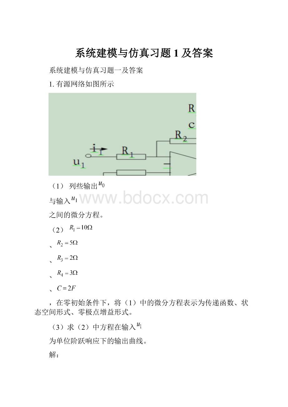
1.有源网络如图所示
(1)列些输出
与输入
之间的微分方程。
(2)
、
、
、
、
,在零初始条件下,将
(1)中的微分方程表示为传递函数、状态空间形式、零极点增益形式。
(3)求
(2)中方程在输入
为单位阶跃响应下的输出曲线。
解:
(1)由运算放大器的基本特点以及电压定理
(3)式代入
(2)式得:
(5)
消去中间变量
有
两边求导整理后得
(2)
代入数据可以得到微分方程为:
程序如下:
clc;clear;
num=[-6.2-0.7];
den=[101];
Gtf=tf(num,den)
Gss=ss(Gtf)
Gzpk=zpk(Gtf)
结果:
Transferfunction:
-6.2s-0.7
------------
10s+1
状态空间形式:
a=
x1
x1-0.1
b=
u1
x10.125
c=
x1
y1-0.064
d=
u1
y1-0.62
Continuous-timemodel.
Zero/pole/gain:
-0.62(s+0.1129)
----------------
(s+0.1)
(3)
由
(2)知系统的传递函数为
-6.2s-0.7
------------
10s+1
系统的输入信号为单位阶跃函数,则其Laplace变换为1/s,这样系统的输出信号的Laplace变换为
Y(s)=
-6.2s-0.7
------------
10s^2+s
编写程序,将其表示为(R,P,Q)形式
clc;clear;
s=tf('s')
Gtf=(-6.2*s-0.7)/(10*s^2+s)
[num,den]=tfdata(Gtf,'v')
[R,P,Q]=residue(num,den)
R=
0.0800
-0.7000
P=
-0.1000
0
Q=
[]
于是得到:
绘制曲线程序:
clc;clear;
t=0:
0.1:
100;
y=0.08*exp(-0.1*t)-0.7;
plot(t,y)
2.已知系统的框图如下:
其中:
G1=1/(s+1),G2=s/(s^2+2),G3=1/s^2,G4=(4*s+2)/(s+1)^2,G5=(s^2+2)/(s^3+14)。
(1)根据梅森公式求总系统传递函数
(2)根据节点、支点、相加点移动方法求总系统传递函数
(3)根据feedback()函数求总系统传递函数
解:
(1)
前向通道传递函数为
三个回路:
,
,
两个不接触回路:
clc;clear;
s=tf('s');
G1=1/(s+1);
G2=s/(s^2+2);
G3=1/s^2;
G4=(4*s+2)/(s+1)^2;
G5=(s^2+2)/(s^3+14);
G=minreal(3*G3*G2*G1/(1+G4*G2*G1+50*G3+G5*G3*G2*G1+50*G3*G4*G2*G1))
结果:
Transferfunction:
3s^6+6s^5+3s^4+42s^3+84s^2+42s
------------------------------------------------------------------------------------------------------------------------------------------
s^10+3s^9+55s^8+175s^7+300s^6+923s^5+2456s^4+3715s^3+2132s^2+2802s+1400
(2)
,
,
构成反馈回路
50,
构成反馈回路
clc;clear;
s=tf('s');
G1=1/(s+1);
G2=s/(s^2+2);
G3=1/s^2;
G4=(4*s+2)/(s+1)^2;
G5=(s^2+2)/(s^3+14);
G124=G2*G1/(1+G2*G1*G4);
G350=G3/(1+G3*50);
G=minreal(3*G350*G124/(1+G350*G124*G5))
结果:
Transferfunction:
3s^6+6s^5+3s^4+42s^3+84s^2+42s
------------------------------------------------------------------------------------------------------------------------------------------
s^10+3s^9+55s^8+175s^7+300s^6+923s^5+2456s^4+3715s^3+2132s^2+2802s+1400
(3)
clc;clear;
s=tf('s');
G1=1/(s+1);
G2=s/(s^2+2);
G3=1/s^2;
G4=(4*s+2)/(s+1)^2;
G5=(s^2+2)/(s^3+14);
G124=feedback(G2*G1,G4);
G350=feedback(G3,50);
G=minreal(3*feedback(G350*G124,G5))
结果:
Transferfunction:
3s^6+6s^5+3s^4+42s^3+84s^2+42s
------------------------------------------------------------------------------------------------------------------------------------------
s^10+3s^9+55s^8+175s^7+300s^6+923s^5+2456s^4+3715s^3+2132s^2+2802s+1400
3.已知系统的传递函数模型为:
(1)采用tf()函数将该传递函数模型输入到MATLAB环境。
(2)采用zpk()、tf2zp()函数将上述传递函数模型转化为零极点增益模型。
(3)采用ss()、tf2ss()函数将上述传递函数模型转化为状态空间模型。
(4)采用tf()、ss2tf()将(3)中变换后的状态空间模型回变为传递函数模型,并与
(1)的结果进行比较。
(5)采用Residue()函数将上述传递函数模型转化为部分分式模型。
(6)绘制系统的零极点图。
解:
(1)
clc;clear;
num=[1042];
den1=conv([101],conv([101],[101]))+[0000025];
den=conv([1,0],conv([1,0],conv([1,0],conv([1,02],den1))));
G=tf(num,den)
结果:
s^3+4s+2
-------------------------------------------------------------------
s^11+5s^9+9s^7+2s^6+12s^5+4s^4+12s^3
(2)
clc;clear;
num=[1042];
den1=conv([101],conv([101],[101]))+[0000025];
den=conv([1,0],conv([1,0],conv([1,0],conv([1,02],den1))));
G=tf(num,den);
sys=zpk(G)
[z,p,k]=tf2zp(num,den)
结果:
(s+0.4735)(s^2-0.4735s+4.224)
-------------------------------------------------------------------------------------------------------
s^3(s^2+1.544s+1.227)(s^2-1.762s+1.755)(s^2+2)(s^2+0.2176s+2.786)
z=
0.2367+2.0416i
0.2367-2.0416i
-0.4735
p=
0
0
0
0.8810+0.9896i
0.8810-0.9896i
-0.7722+0.7940i
-0.7722-0.7940i
-0.1088+1.6657i
-0.1088-1.6657i
-0.0000+1.4142i
-0.0000-1.4142i
k=
1
(3)
clc;clear;
num=[1042];
den1=conv([101],conv([101],[101]))+[0000025];
den=conv([1,0],conv([1,0],conv([1,0],conv([1,02],den1))));
G=tf(num,den);
sys=ss(G)
[A,B,C,D]=tf2ss(num,den)
结果:
a=
x1x2x3x4x5x6x7x8x9x10
x10-1.250-1.125-0.25-0.75-0.25-0.7500
x24000000000
x30200000000
x40010000000
x50001000000
x60000200000
x70000010000
x80000001000
x90000000100
x100000000020
x110000000000.5
x11
x10
x20
x30
x40
x50
x60
x70
x80
x90
x100
x110
b=
u1
x10.5
x20
x30
x40
x50
x60
x70
x80
x90
x100
x110
c=
x1x2x3x4x5x6x7x8x9x10x11
y100000000.12500.250.25
d=
u1
y10
Continuous-timemodel.
A=
0-50-9-2-12-4-12000
10000000000
01000000000
00100000000
00010000000
00001000000
00000100000
00000010000
00000001000
00000000100
00000000010
B=
1
0
0
0
0
0
0
0
0
0
0
C=
00000001042
D=
0
(4)
clc;clear;
num=[1042];
den1=conv([101],conv([101],[101]))+[0000025];
den=conv([1,0],conv([1,0],conv([1,0],conv([1,02],den1))));
G=tf(num,den);
sys=ss(G);
[A,B,C,D]=tf2ss(num,den);
sys=tf(sys)
[num,den]=ss2tf(A,B,C,D)
结果:
Transferfunction:
s^3-1.11e-016s^2+4s+2
---------------------------------------------------------------------------------------------------------------------------
s^11+4.816e-015s^10+5s^9+2.386e-014s^8+9s^7+2s^6+12s^5+4s^4+12s^3
num=
Columns1through9
00.000000.0000-0.00000.00000.0000-0.00001.0000
Columns10through12
0.00004.00002.0000
den=
Columns1through9
1.0000-0.00005.00000.00009.00002.000012.00004.000012.0000
Columns10through12
000
(5)
clc;clear;
num=[1042];
den1=conv([101],conv([101],[101]))+[0000025];
den=conv([1,0],conv([1,0],conv([1,0],conv([1,02],den1))));
[R,P,Q]=residue(num,den)
结果:
R=
-0.0246+0.0089i
-0.0246-0.0089i
0.0833+0.0295i
0.0833-0.0295i
0.0274+0.0298i
0.0274-0.0298i
0.0435+0.0581i
0.0435-0.0581i
-0.2593
0.2778
0.1667
P=
-0.1088+1.6657i
-0.1088-1.6657i
-0.0000+1.4142i
-0.0000-1.4142i
0.8810+0.9896i
0.8810-0.9896i
-0.7722+0.7940i
-0.7722-0.7940i
0
0
0
Q=
[]
(6)
clc;clear;
num=[1042];
den1=conv([101],conv([101],[101]))+[0000025];
den=conv([1,0],conv([1,0],conv([1,0],conv([1,02],den1))));
G=tf(num,den);
pzmap(G)
结果:
4.考虑二阶系统:
系统的输入为
。
(1)利用部分分式模型方法求输出的解析解
,并绘制其曲线。
(2)利用lsim(G,u,t)函数直接绘制系统的输出曲线,并与
(1)的结果比较。
解:
(1)
先求
的Laplace变换
clc;clear;
symst
f=sin(2*t);
F=laplace(f)
结果:
F=
2/(s^2+4)
于是:
以下求
的部分分式模型:
clc;clear;
s=tf('s');
G=2/((s^2+2*s+1)*(s^2+4));
[num,den]=tfdata(G,'v');
[R,P,Q]=residue(num,den)
R=
-0.0800+0.0600i
-0.0800-0.0600i
0.1600
0.4000
P=
0.0000+2.0000i
0.0000-2.0000i
-1.0000
-1.0000
Q=
[]
可以得到解析解为:
绘制曲线:
clc;clear;
t=0:
0.1:
50;
y=(-0.0800+0.0600*i)*exp(2*i*t)+(-0.0800-0.0600*i)*exp(-2*i*t)+0.16*exp(-t)+0.4*t.*exp(-t);
plot(t,y)
(2)
clc;clear;
t=0:
0.1:
50;
s=tf('s');
G=1/(s^2+2*s+1);
u=sin(2*t)
lsim(G,u,t)
讨论:
在
(1)中得到解析解为:
这个结果前半部分物理意义不能直接表达出来。
如果采用以下变换:
式中:
,
,则可以得出解析解的更简明的形式。
编写以下通用程序:
文件名为bianhuan.m
function[R,P,Q]=bianhuan(num,den)
[R,P,Q]=residue(num,den);
fork=1:
length(R)
ifimag(P(k))>eps
a=real(R(k));b=imag(R(k));
R(k)=-2*sqrt(a^2+b^2);R(k+1)=-atan2(a,b);
elseifabs(imag(P(k)))R(k)=real(R(k));
end
end
如果P(k)为实数,则(R(k),P(k))对和标准的residue()函数中定义是完全一致的。
如果P(k)为复数,则(R(k),R(k+1))对返回
和
参数,而P(k)的定义仍与residue()中的一致。
以下编写程序,调用程序调用bianhuan.m,将解析解:
用正弦以及指数的形式表示。
clc;clear;
s=tf('s');
G=2/((s^2+2*s+1)*(s^2+4));
[num,den]=tfdata(G,'v');
[R,P,Q]=bianhuan(num,den)
结果:
R=
-0.2000
0.9273
0.1600
0.4000
P=
0.0000+2.0000i
0.0000-2.0000i
-1.0000
-1.0000
Q=
[]
于是解析式可以写为:
5.假设离散系统的传递函数为:
,
将该传递函数模型输入到MATLAB环境;将上述传递函数模型转化为零极点增益模型;将上述传递函数模型转化为状态空间模型;采用Residue()函数将上述传递函数模型转化为部分分式模型。
解:
clc;clear;
num=[100.568];
den=[1-1.21.19-0.99];
G=tf(num,den,0.1)
[z,p,k]=tf2zp(num,den);
G=zpk(z,p,k,0.1)
[A,B,C,D]=tf2ss(num,den);
G=ss(A,B,C,D,0.1)
[R,P,Q]=residue(num,den)
结果:
Transferfunction:
z^2+0.568
-----------------------------
z^3-1.2z^2+1.19z-0.99
Samplingtime:
0.1
Zero/pole/gain:
(z^2+0.568)
--------------------------
(z-1)(z^2-0.2z+0.99)
Samplingtime:
0.1
a=
x1x2x3
x11.2-1.190.99
x2100
x3010
b=
u1
x11
x20
x30
c=
x1x2x3
y1100.568
d=
u1
y10
Samplingtime:
0.1
Discrete-timemodel.
R=
0.8760
0.0620-0.1574i
0.0620+0.1574i
P=
1.0000
0.1000+0.9899i
0.1000-0.9899i
Q=
[]
 升级会员
升级会员 