信号与系统实验.docx
《信号与系统实验.docx》由会员分享,可在线阅读,更多相关《信号与系统实验.docx(11页珍藏版)》请在冰豆网上搜索。
信号与系统实验
第2章信号的时域分析
M2-2
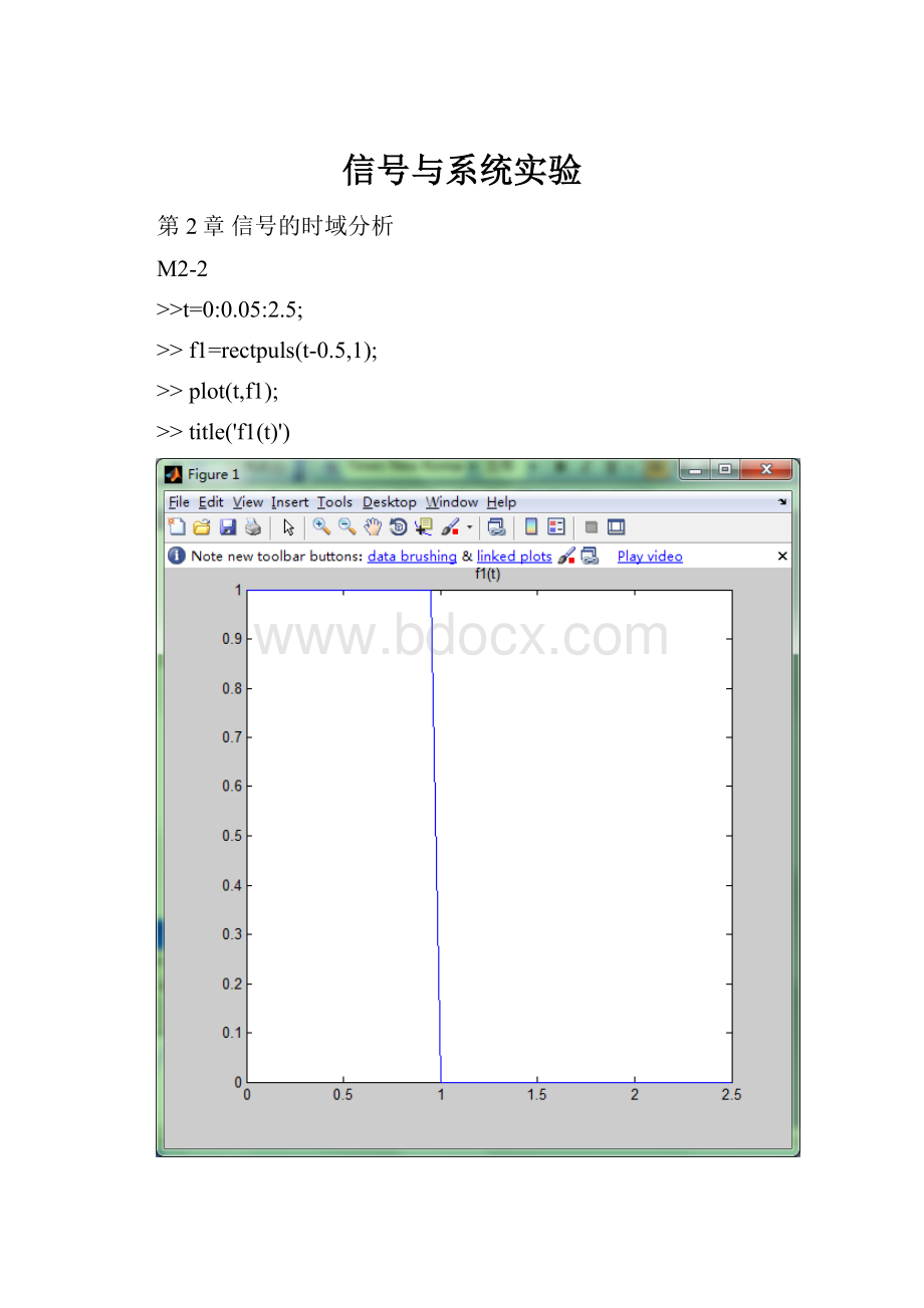
>>t=0:
0.05:
2.5;
>>f1=rectpuls(t-0.5,1);
>>plot(t,f1);
>>title('f1(t)')
>>f2=tripuls(t-1,2,0);
>>plot(t,f2)
>>title('f2(t)')
plot(t,f2.*cos(50*t))
>>title('f2(t)cos(50t)')
>>f=f1+f2.*cos(50*t)
f=
Columns1through12
1.00000.95991.02841.05200.83221.24940.77211.07681.16320.60701.49560.6068
Columns13through24
1.09261.30400.36741.73520.46641.07511.47280.11640.9650-0.58520.01990.4935
Columns25through36
-0.76190.7091-0.3937-0.02870.3800-0.53380.4609-0.2279-0.04420.2391-0.29530.2235
Columns37through48
-0.0896-0.02640.0730-0.049700000000
Columns49through51
000
>>plot(t,f);
>>title('f(t)')
M2-4
(1)>>t=-5:
0.001:
6;
>>f=rectpuls(t+0.5,1)+(1-t).*rectpuls(t-0.5,1)-rectpuls(t-1.5,1);
>>plot(t,f)
>>title('f(t)');
(2)
>>f1=rectpuls(0.5*t+0.5,1)+(1-0.5*t).*rectpuls(0.5*t-0.5,1)-rectpuls(0.5*t-1.5,1);
>>plot(t,f1);
>>title('f(0.5t)');
>>f2=rectpuls(2-0.5*t+0.5,1)+(1-2+0.5*t).*rectpuls(2-0.5*t-0.5,1)-rectpuls(2-0.5*t-1.5,1);
>>plot(t,f2);
>>title('f(2-0.5t)');
M2-8
>>t=-pi/3:
pi/1000:
pi/3;
>>g1=cos(6*pi*t);
>>k=-10:
10;
>>f1=cos(6*pi*k/10);
>>subplot(3,1,1);
>>plot(t,g1,k/10,f1)
>>title('g1(t)')
>>g2=cos(14*pi*t);
>>f2=cos(14*pi*k/10);
>>subplot(3,1,2);
>>plot(t,g2,k/10,f2)
>>title('g2(t)')
>>g3=cos(26*pi*t);
>>f3=cos(26*pi*k/10);
>>subplot(3,1,3);
>>plot(t,g3,k/10,f3)
>>title('g3(t)')
讨论:
频率越大,波形越密集,对于相同的采样频率,每个波形周期内采样点则越少,采样失真越严重,更不能反映原波形。
第3章系统的时域分析
M3-2
(1)L(1/R1+1/R2)d2y(t)/dt2+(L/R1R2C+1)dy(t)/dt+1/(R2C)y(t)=df(t)/dt
代入数值得
1.5d2y(t)/dt2+1.5dy(t)/dt+0.5y(t)=df(t)/dt
(2)
>>ts=0;te=12;dt=0.01;
>>sys=tf([1],[1.51.50.5]);
>>t=ts:
dt:
te;
>>y=impulse(sys,t);
>>plot(t,y);
>>xlabel('Time(sec)')
>>ylabel('y(t)')
(3)
>>y=step(sys,t);
>>plot(t,y);
>>xlabel('Time(sec)')
>>ylabel('y(t)')
 升级会员
升级会员 