黑色星期五的数据探索分析EDA 实战.docx
《黑色星期五的数据探索分析EDA 实战.docx》由会员分享,可在线阅读,更多相关《黑色星期五的数据探索分析EDA 实战.docx(19页珍藏版)》请在冰豆网上搜索。
黑色星期五的数据探索分析EDA实战
1.前置知识
什么黑色星期五?
黑色星期五可以简单理解为国外的双十一,指十一月第四个星期五,各商场都会推出量的打折和优惠活动的日子。
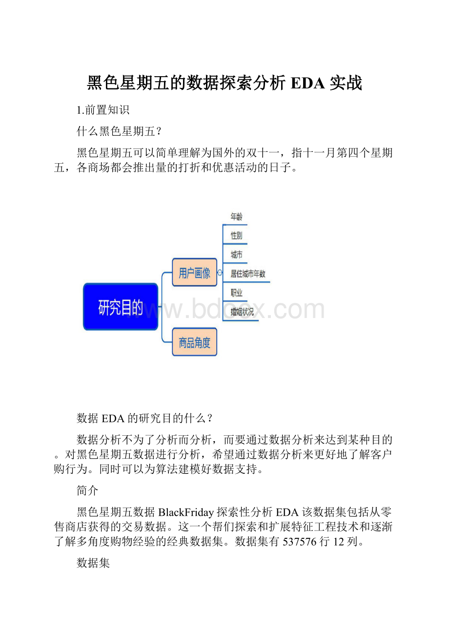
数据EDA的研究目的什么?
数据分析不为了分析而分析,而要通过数据分析来达到某种目的。
对黑色星期五数据进行分析,希望通过数据分析来更好地了解客户购行为。
同时可以为算法建模好数据支持。
简介
黑色星期五数据BlackFriday探索性分析EDA该数据集包括从零售商店获得的交易数据。
这一个帮们探索和扩展特征工程技术和逐渐了解多角度购物经验的经典数据集。
数据集有537576行12列。
数据集
见文件数据集有537576行12列
环境需求
Anaconda2+pycharm+numpy+pandas+matplotlib+scikitlearn+RF
运行结果
代码实现:
#TODO:
BlackFridayEDA
#关于一家零售店黑色星期五的55万次观测数据
#它包含不同类型的变量,无论数值变量还类别型变量
#todo:
1.Libraies
#们将会使用Pandas,Numpy,Seaborn和Matplotlib库进行分析
#Warnings
importwarnings
warnings.filterwarnings("ignore")
importpandasaspd
importnumpyasnp
#可视化
importseabornassns
importmatplotlib.pyplotasplt
importos
#printos.listdir("E:
\Python\BlackFriday")#Toreturnthe
whichfileslistcontaindec
sns.set(style="darkgrid")
#plt.rcParams["patch.force_edgecolor"]=True#matplotlib
中rcParams主要用来设置图像像素,画图的分辨率,小等信息
#patch.force_edgecolor打全球的边缘
#TODO:
数据加载与特征提取
df=pd.read_csv("BlackFriday.csv")
#printdf.head
(2)
#User_IDProduct_IDGenderAgeOccupation
City_Category\
#01000001P00069042F0-1710
A
#11000001P002442F0-1710
A
#
#Stay_In_Current_City_YearsMarital_Status
Product_Category_1\
#020
3
#120
1
#
#Product_Category_2Product_Category_3Purchase
#0NaNNaN8370
#16.014.015200
#printdf.info()
#printdf.shape
#RangeIndex:
537577entries,0to537576
#Datacolumns(total12columns):
#User_ID537577non-nullint64
#Product_ID537577non-nullobject
#Gender537577non-nullobject
#Age537577non-nullobject
#Occupation537577non-nullint64
#City_Category537577non-nullobject
#Stay_In_Current_City_Years537577non-nullobject
#Marital_Status537577non-nullint64
#Product_Category_1537577non-nullint64
#Product_Category_2370591non-nullfloat64
#Product_Category_3164278non-nullfloat64
#Purchase537577non-nullint64
#dtypes:
float64
(2),int64(5),object(5)
#memoryusage:
49.2+MB
#None
#(537577,12)
#TODO:
缺失值的处理
total_miss=df.isnull().sum()#对应特征缺失值总数
#printtotal_miss
#User_ID0
#Product_ID0
#Gender0
#Age0
#Occupation0
#City_Category0
#Stay_In_Current_City_Years0
#Marital_Status0
#Product_Category_10
#Product_Category_2166986
#Product_Category_3373299
#Purchase0
#dtype:
int64
#printtotal_miss
per_miss=total_miss/df.isnull().count()#每列对应特征
的nan数/所有特征nan乘以100对应特征的缺失比值
#printtotal_miss/df.isnull().count()*100#每列对应特征的
nan数/所有特征nan乘以100
#User_ID0.000000
#Product_ID0.000000
#Gender0.000000
#Age0.000000
#Occupation0.000000
#City_Category0.000000
#Stay_In_Current_City_Years0.000000
#Marital_Status0.000000
#Product_Category_10.000000
#Product_Category_231.062713
#Product_Category_369.441029
#Purchase0.000000
#dtype:
float64
missing_data=pd.DataFrame({'Totalmissing':
total_miss,
'%missing':
per_miss})
#printmissing_data
#printmissing_data.sort_values(by='Total
missing',ascending=False).head(3)
#%missingTotalmissing
#Product_Category_30.694410373299
#Product_Category_20.310627166986
#User_ID0.0000000
#由于多数产品只属于一个类别,所以少一些产品有第二个类别
有意义的,更不用说第三个类别了。
#TODO:
值
#探讨数据中特征中的值。
总共有537577
#print"UniqueValuesforEachFeature:
\n"
#printdf.columns
#Index([u'User_ID',u'Product_ID',u'Gender',u'Age',
u'Occupation',
#u'City_Category',u'Stay_In_Current_City_Years',
u'Marital_Status',
#u'Product_Category_1',u'Product_Category_2',
u'Product_Category_3',
#u'Purchase'],
#dtype='object')
#foriindf.columns:
#i对应就columns中的每一列
#printi,':
',df[i].unique()
#todo:
关于产品信息
#print"Numberofproducts:
",df['Product_ID'].unique()
#print"Numberofproducts
Numbers:
",len(df['Product_ID'].unique().tolist())
#print"Numberof
categories:
",df["Product_Category_1"].unique().max()
#print"Highestandlowest
purchase:
",df['Purchase'].max(),',',df['Purchase'].min()
#Numberofproducts:
['P00069042''P002442'
'P00087842'...,'P00038842''P00295642'
#'P00091742']
#NumberofproductsNumbers:
3623
#Numberofcategories:
18
#Highestandlowestpurchase:
23961,185
#todo:
关于家信息
#print"Numberofshoppers:
",df['User_ID'].unique()
#print"Shoppers数
量:
",len(df['User_ID'].unique().tolist())
#print"Yearsin
city:
",df['Stay_In_Current_City_Years'].unique()
#print"AgeGroup:
",df['Age'].unique()
#Numberofshoppers:
[100000110000021000003...,1004113
10053911001529]
#Shoppers数量:
51
#Yearsincity:
['2''4+''3''1''0']
#AgeGroup:
['0-17''55+''26-35''46-50''51-55''36-45'
'18-25']
#TODO:
Gender
#首先,通过查看每个条目的数量来确定数据否按性别均匀分布;
count_m=df[df['Gender']=='M']#在DataFrame中选择性别为M
的所有数据
#printdf['Gender']=='M'
#printcount_m
count_m_count=df[df['Gender']=='M'].count()
count_m_count=df[df['Gender']=='M'].count()[0]
#printcount_m_count
#User_ID405380
#Product_ID405380
#Gender405380
#Age405380
#Occupation405380
#City_Category405380
#Stay_In_Current_City_Years405380
#Marital_Status405380
#Product_Category_1405380
#Product_Category_2280741
#Product_Category_3127346
#Purchase405380
#dtype:
int64
#User_IDProduct_IDGenderAgeOccupation
City_Category\
#41000002P00285442M55+16
C
#51000003P00193542M26-3515
A
#61000004P00184942M46-507
B
#71000004P00346142M46-507
B
#81000004P0097242M46-507
B
#91000005P00274942M26-3520
A
#print
"count_m_count=df[df['Gender']=='M'].count()[0]:
",df[df['Ge
nder']=='M'].count()[0]
#count_m_count=df[df['Gender']=='M'].count()[0]:
405380
count_f=df[df['Gender']=='F'].count()[0]
print"Numberofmaleclients:
",count_m_count
print"Numberoffemaleclients:
",count_f
#男客户数量:
405380
#女客户数量:
132197
#们可以看到记录的男性客户数量超过4次记录的女性客户数量。
因此,通过使用比率而不计算每条数据来分析性别将更加信息化。
让们看看每个性别的多少每个人均消费
print"Female
Purchases:
",round(df[df["Gender"]=='F']['Purchase'].sum()/c
ount_f)
print"Male
Purchases:
",round(df[df["Gender"]=='M']['Purchase'].sum()/c
ount_m_count)
#FemalePurchases:
8809.0女性人均消费
#MalePurchases:
9504.0男性分均消费
#图形绘制
#nunique()Returnnumberofuniqueelementsintheobject.
plt.pie(df.groupby('Gender')['Product_ID'].nunique(),labels
=['Male','Female'],
shadow=True,
autopct='%1.1f%%',colors=['steelblue','cornflowerblue'])
plt.title('UniqueItemPurchasesbyGender')
plt.show()
printdf.groupby('Gender')['Product_ID'].nunique()
#F3358
#M3582
#Name:
Product_ID,dtype:
int64
#虽然差不多,但女性确实购了比男性更多的产品。
现在,让们
根据产品类别分析每个性别购的比例。
#按照性别进行分组
print"===================="
#printdf[df['Gender']=='M']
#User_IDProduct_ID...Product_Category_3
Purchase
#41000002P00285442...NaN
7969
#51000003P00193542...NaN
15227
#61000004P00184942...17.0
19215
#71000004P00346142...NaN
15854
gender=df[df['Gender']=='M'][['Product_Category_1',
'Gender']]#针对过滤为男性用户的数据进行选取
Product_Category_1Gender
#printgender
#Product_Category_1Gender
#48M
#51M
#61M
#todo:
品类1中的男性用户数量
gb_gender_m=df[df['Gender']=='M'][['Product_Category_1',
'Gender']].count()
print"gb_gender_m:
\n",gb_gender_m
gb_gener_f=df[df['Gender']=='F'][['Product_Category_1',
'Gender']].count()
#print"gb_gender_f:
\n",gb_gener_f
#gb_gender_m:
#Product_Category_1405380
#Gender405380
#dtype:
int64
#gb_gender_f:
#Product_Category_1132197
#Gender132197
#连接并更改列名称
print"---------------------------------"
cat_bygender=pd.concat([gb_gender_m,gb_gener_f],axis=1)
#printcat_bygender
#01
#Product_Category_1405380132197
#Gender405380132197
cat_bygender.columns=['Mratio','Fratio']
#printcat_bygender
#MratioFratio
#Product_Category_1405380132197
#Gender405380132197
#调整以比率
cat_bygender['Mratio']=cat_bygender['M
ratio']/df[df['Gender']=='M'].count()[0]
cat_bygender['Fratio']=cat_bygender['F
ratio']/df[df['Gender']=='F'].count()[0]
#printdf[df['Gender']=='M'].count()
#User_ID405380
#Product_ID405380
#Gender405380
#Age405380
#Occupation405380
#City_Category405380
#Createlikelihoodofonegendertobuyovertheother
cat_bygender['Likelihood(M/F)']=cat_bygender['M
ratio']/cat_bygender['Fratio']
cat_bygender['TotalRatio']=cat_bygender['M
ratio']+cat_bygender['Fratio']
cat_bygender.sort_values(by='Likelihood
(M/F)',ascending=False)
#printcat_bygender
#TODO:
Age
#Age值字符串,们现在对每个组进行编码,以便它们可以用机
器学习算法可以理解的整数值表示
#年龄组编码
df['Age_Encoded']=df['Age'].map({'0-17':
0,'18-25':
1,
'26-35':
2,'36-45':
3,
'46-50':
4,'51-55':
5,
'55+':
6})
prod_byage=df.groupby('Age').nunique()['Product_ID']
fig,ax=plt.subplots(1,2,figsize=(14,6))
ax=ax.ravel()
sns.countplot(df['Age'].sort_values(),ax=ax[0],
palette="Blues_d")
ax[0].set_xlabel('AgeGroup')
ax[0].set_title('AgeGroupDistribution')
sns.barplot(x=prod_byage.index,y=prod_byage.values,ax=ax[1]
palette="Blues_d")
ax[1].set_xlabel('AgeGroup')
ax[1].set_title('UniqueProductsbyAge')
plt.show()
#很明显,客户中的年龄组26-35岁。
有趣的,就数量而言,
产品购的分布在各年龄组之间差异不。
这意味着,虽然26-35
岁年龄组的,但其他年龄组购的几乎与他们一样多。
但
这否意味着在年龄组中花费的金额相同的?
让们来看一下
spent_byage=df.groupby(by='Age').sum()['Purchase']
plt.figure(figsize=(12,6))
sns.barplot(x=spent_byage.index,y=spent_byage.values,
palette="Blues_d")
plt.title('MeanPurchasesperAgeGroup')
plt.show()
#们的数据清楚地表明,每个年龄组的资金数额与年龄组内的客户
数量成正比。
这可能商店的有价值的信息,因为它可能希望在未
来更多针对该年龄组的产品,或者可能致力于营销不同的以
增加其客户年龄组的更广泛的多样性。
#TODO:
Occupation
#Thissectionsdrawssomeinsightsonourdataintermsofthe
occupationofthecustomers.
plt.figure(figsize=(12,6))
sns.countplot(df['Occupation'])
plt.title('OccupationDistribution')
plt.show()
plt.figure(figsize=(12,6))
prod_by_occ=
df.groupby(by='Occupation').nunique()['Product_ID']
sns.barplot(x=prod_by_occ.index,y=prod_by_occ.values)
plt.title('UniqueProductsbyOccupation')
plt.show()
spent_by_occ=df.groupby(by='Occupation').sum()['Purchase']
plt.figure(figsize=(12,6))
sns.barplot(x=spent_by_occ.index,y=spent_by_occ.values)
plt.title('TotalMoneySpentperOccupation')
plt.show()
#再一次,每个职业所花费的平均金额的分配似乎反映了每个职业中
人数的分布。
从数据科学的角度来看,这幸运的,因为们没有
使用奇怪或突出的功能。
们在年龄和职业方面的数据似乎很有意
义。
#TODO:
Products
#这里,们探索产品本身。
这很重要,因为们在此数据集中没有
标记的。
从理论上讲,客户可以在4台新电视或10,000支笔上
花费5,000美元。
这种差异对商店很重要,因为他们的利润受到影
响。
由于们不知道这些什么,让们探索的类别。
plt.figure(figsize=(12,6))
prod_by_cat=
df.groupby('Product_Category_1')['Product_ID'].nunique()
sns.barplot(x=prod_by_cat.index,y=prod_by_cat.values,
palette="Blues_d")
plt.title('NumberofUniqueItemsperCategory')
plt.show()
#类别标签1,5和8显然具有最多的。
这可能意味着商店以该项
目而闻名,或者该类别广泛的。
category=[]
mean_purchase=[]
foriindf['Product_Category_1'].unique():
category.append(i)
cate
 升级会员
升级会员 