计量经济学期末课程论文范文Word下载.doc

计量经济学期末课程论文范文Word下载.doc

《计量经济学期末课程论文范文Word下载.doc》由会员分享，可在线阅读，更多相关《计量经济学期末课程论文范文Word下载.doc（6页珍藏版）》请在冰豆网上搜索。

42361

910.9

107.5

1981

4891.6

43725

961

102.5

1982

5323.4

45295

1230.4

102

1983

5962.7

46436

1430.1

1984

7208.1

48197

1832.9

102.7

1985

9016

49873

2543.2

109.3

1986

10275.2

51282

3120.6

106.5

1987

12058.6

52783

3791.7

107.3

1988

15042.8

54334

4753.8

118.8

1989

16992.3

55329

4410.4

118

1990

18667.8

64749

4517

103.1

1991

21781.5

65491

5594.5

103.4

1992

26923.5

66152

8080.1

106.4

1993

35333.9

66808

13072.3

114.7

1994

48197.9

67455

17042.1

124.1

1995

60793.7

68065

20019.3

117.1

1996

71176.6

68950

22913.5

108.3

1997

78973

69820

24941.1

102.8

1998

84402.3

70637

28406.2

99.2

1999

89677.1

71394

29854.7

98.6

2000

99214.6

72085

32917.7

100.4

2001

109655.2

73025

37213.5

100.7

2002

120332.7

73740

43499.9

2003

135822.8

74432

55566.6

101.2

2004

159878.3

75200

70477.4

103.9

2005

184937.4

75825

88773.6

101.8

2006

216314.4

76400

109998.2

101.5

2007

265810.3

76990

137323.9

104.8

2008

314045.4

77480

172828.4

105.9

2009

340903

77995

224598.8

99.3

资料来源：

中经网统计数据库。

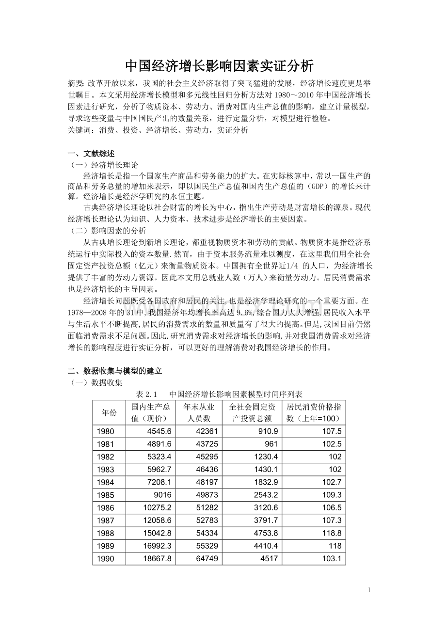
（二）模型设计

为了具体分析各要素对我国经济增长影响的大小，我们可以用国内生产总值（y）作为对经济发展的衡量，代表经济发展；

用总就业人员数（x1）衡量劳动力；

用固定资产投资总额（x2）衡量资本投入：

用价格指数（x3）去代表消费需求。

运用这些数据进行回归分析。

采用的模型如下：

y=β1+β2x1+β3x2+β4x3+ui

其中，y代表国内生产总值，x1代表社会就业人数，x2代表固定资产投资，x3代表消费价格指数，ui代表随机扰动项。

我们通过对该模型的回归分析，得出各个变量与我国经济增长的变动关系。

三、模型估计和检验

（一）模型初始估计

表3.1模型初始估计结果

DependentVariable:

Y

Method:

LeastSquares

Date:

06/07/11Time:

16:

33

Sample（adjusted）:

19802009

Includedobservations:

30afteradjustingendpoints

Variable

Coefficient

Std.Error

t-Statistic

Prob.

C

-16197.47

41510.11

-0.390205

0.6996

X1

1.683972

0.256065

6.576336

0.0000

X2

1.420445

0.054886

25.87979

X3

-580.7369

355.4395

-1.633856

0.1143

R-squared

0.985665

Meandependentvar

85805.26

AdjustedR-squared

0.984011

S.D.dependentvar

95097.07

S.E.ofregression

12024.95

Akaikeinfocriterion

21.75092

Sumsquaredresid

3.76E+09

Schwarzcriterion

21.93775

Loglikelihood

-322.2638

F-statistic

595.9008

Durbin-Watsonstat

0.968679

Prob（F-statistic）

0.000000

（二）多重共线性检验

表3.2相关系数矩阵

1.000000

0.665094

-0.219318

1.000000

-0.291137

根据多重共线性检验，解释变量之间存在着线性相关。

通过采用剔除变量法，多重共线性的修正结果如下：

剔除X3。

.

表3.3修正多重共线性后的模型

40

-79282.79

15704.05

-5.048555

1.699013

0.263693

6.443158

1.438325

0.055422

25.95222

0.984193

Meandependentvar

0.983022

S.D.dependentvar

12391.14

Akaikeinfocriterion

21.78199

4.15E+09

Schwarzcriterion

21.92211

-323.7299

F-statistic

840.5434

0.689221

Prob（F-statistic）

（三）异方差检验

表3.4ARCH检验

ARCHTest:

F-statistic

5.690752

Probability

0.024334

Obs*R-squared

5.048272

0.024651

TestEquation:

RESID^2

44

19812009

29afteradjustingendpoints

49385817

56010198

0.881729

0.3857

RESID^2（-1）

0.899098

0.376897

2.385530

0.0243

0.174078

1.39E+08

0.143489

2.41E+08

2.23E+08

41.35408

1.35E+18

41.44838

-597.6342

1.336249

从上表可以得到数据：

（n-p）R2=5.048272,查表得χ2（p）=5.9915,（n-p）R2=5.048272<

χ2（p）=5.9915,则接受原假设，不存在异方差。

（四）序列相关检验

已知：

DW=0.689221，查表得dL=1.270，dU=1.563。

由此可知，存在相关性。

修正如下：

表3.5修正序列相关后的模型

DependentV